8 Analysis of Functions with Two Variables
\[ \definecolor{dgray}{rgb}{0.3,0.3,0.3} \definecolor{lgray}{rgb}{0.85,0.85,0.85} \]
8.1 Preliminary Remarks
In this chapter, we will further develop and extend to functions of two variables the methods of differential calculus presented in Chapter 3.
What can we expect?
The familiar formulas for differentiating powers, logarithms, and exponential functions still apply. The same is true for the rules we are just as familiar with, such as the product rule, chain rule, etc.
What’s changing?
Our functions now involve two independent variables. Whereas the graphs of functions of one variable were curves in the plane, the graphs are now generally more or less complexly shaped surfaces in 3-dimensional space. Therefore, we have changed the geometric context, which we must account for in an appropriate way.
Hence, it is only logical to begin by discussing some important geometric foundations.
8.2 Geometric Foundations
We will usually denote the independent variables of the functions we consider with \(x\) and \(y\). Geometrically, they correspond to the coordinates of a point \(\mathbf x=\left(\begin{array}{c}x\\y\end{array}\right)\) in the \((x,y)\)-plane, in \(\mathbb R^2\). While in functions of one variable these take their values in a one-dimensional interval, \(\mathbf x\) can now be any point of a subset \(M\subset\mathbb R^2\).
However, we will frequently and with good reason stipulate that the coordinates \(x\) and \(y\) of the point \(\mathbf x\) are not independent of each other, but vary together. By this, we mean that \(x\) and \(y\) are functions of a real variable \(t\): \[ \begin{gathered} x=g_1(t),\quad y=g_2(t),\qquad t\in \mathbb R. \end{gathered} \tag{8.1}\] When the values of \(t\) traverse an interval, \(x\) and \(y\) describe a curve in the plane, which is called a path, parameterized by the equations (8.1).

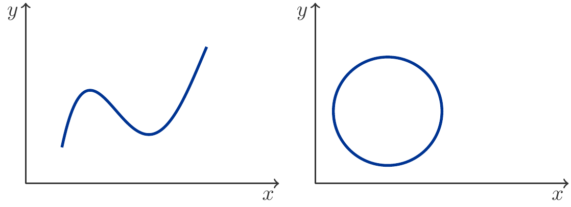
In Figure 8.1, two paths can be seen. The left image shows a path generated by a polynomial of the 3rd degree, \[ \begin{gathered} x=t,\quad y=a_0+a_1t+a_2t^2+a_3t^3,\qquad u\le t\le v \end{gathered} \] whereas in the second example the path is a closed curve (a circle) generated by \[ \begin{gathered} x=a+r\cos t,\quad y=b+r\sin t,\qquad -\pi\le t\le \pi. \end{gathered} \] Here, \(a\) and \(b\) are the coordinates of the center and \(r\) its radius1.
Of course, we are primarily interested in paths that have particularly simple shapes. By this, we mean paths that run straight in \(\mathbb R^2\).

Such lines can be described by linear equations, which readers will surely remember from Chapter 1.
Axis-parallel lines are described by the equations: \[ \begin{gathered} \begin{array}{ccccl} x&=&a &&\text{parallel to the $y$-axis}\\ y&=&b &&\text{parallel to the $x$-axis} \end{array}, \end{gathered} \] Lines in general position by the equation \(ax+by=c\).
It will prove advantageous to have a common description for these three cases. For this purpose, we use the idea of the vector.
We first encountered vectors in Chapter 6. There, we defined them as lists of numbers. We stick to this definition, but limit it to lists of length 2.
Vectors \(\mathbf a,\;\mathbf b\in\mathbb R^2\) can be geometrically interpreted as points or as displacements (symbolized by arrows) (see Figure 8.3).

Calculations with vectors also correspond to geometrical processes.
When you add a displacement vector \(\mathbf v\) to a point vector \(\mathbf p\), the result \(\mathbf q=\mathbf p+\mathbf v\) is that point vector that emerges from the displacement \(\mathbf v\) of the point \(\mathbf p\): \[ \begin{gathered} \text{Starting point} + \text{Displacement}=\text{Endpoint}\\ \mathbf p+\mathbf v=\mathbf q \end{gathered} \]
Accordingly, \(\mathbf v=\mathbf q-\mathbf p\) is the displacement vector from \(\mathbf p\) to \(\mathbf q\): \[ \begin{gathered} \text{Displacement}=\text{Endpoint}-\text{Starting point}\\ \mathbf v = \mathbf q-\mathbf p \end{gathered} \]
Viewed in this way, every point vector \(\mathbf x\) can also be interpreted as a displacement vector from the origin \(\boldsymbol{0}\) of the coordinate system to the point \(\mathbf x\).
Multiplication of a vector by a number is geometrically most easily interpreted through the interpretation of the vector as a displacement vector.
Let \(\mathbf w=\lambda\mathbf v\). The factor \(\lambda\) changes the displacement \(\mathbf v\) in two ways. The sign of \(\lambda\) determines the direction:
If \(\lambda>0\), then \(\mathbf w\) is a displacement in the same direction as \(\mathbf w\).
If \(\lambda<0\), then \(\mathbf w\) is a displacement in the opposite direction from \(\mathbf v\).
The absolute value of \(\lambda\) determines the change in the length of the displacement vector.
Two vectors that differ only by a factor are called proportional. In the interpretation as displacement vectors, proportional thus means nothing other than parallel.
8.2.1 Parametric form of a line
Lines in \(\mathbb R^2\) can be specified by a point \(\mathbf a\) and a displacement vector \(\mathbf v\). Specifically:
Definition 8.1 (Parametric Form of a Line) One calls \[ \begin{gathered} g=\{\mathbf x : \mathbf x = \mathbf a + t\mathbf v, t\in\mathbb R\},\quad \mathbf x=\left(\begin{array}{c}x\\y\end{array}\right), \mathbf v\ne \boldsymbol{0} \end{gathered} \] the parametric form of a line.
Here: \[ \begin{array}{ccl} g &=& \text{Set of all points $x$ on the line}\\ \mathbf x &=& \text{Point on $g$,} \\ \mathbf a &=& \text{Starting point,}\\ \mathbf v &=& \text{Direction vector.} \end{array} \]
Remark 8.2 Of course, there are infinitely many different parametric forms of the same line, depending on which points \(\mathbf a\) and direction vectors \(\mathbf v\) one uses. The resulting set of points is always the same.
One can illustrate the differences between various parametric forms of a line in the following way.
Imagine we start a journey along the line \(g\), where \(\mathbf a\) is the starting point and the parameter \(t\) denotes the elapsed time. When a time span of length \(t=1\) elapses, our position on the line changes by the direction vector \(\mathbf v\). Therefore, the direction vector \(\mathbf v\) is also called the velocity vector.
A parametric form \(\mathbf x=\mathbf a+t\mathbf v\) of a line is thus a uniform motion along the line, starting at point \(\mathbf a\) and proceeding with the velocity vector \(\mathbf v\).
Exercise 8.3 Find a parametric form of the line with the equation \(3x+y=15\).
Solution: We find two points on the line, for example by setting \(x=0\) once and \(y=0\) once: \[ \begin{gathered} \mathbf a=\left(\begin{array}{r}0\\15\end{array}\right),\qquad \mathbf b=\left(\begin{array}{r}5\\0\end{array}\right). \end{gathered} \] Therefore, the corresponding translation vector is: \[ \begin{gathered} \mathbf v=\mathbf b-\mathbf a=\left(\begin{array}{r}5\\-15 \end{array}\right), \end{gathered} \] and a parametric equation of the line thus is: \[ \begin{gathered} g=\left\{\mathbf x=\mathbf a+t\mathbf v= \left(\begin{array}{r}0\\15\end{array}\right) +t \left(\begin{array}{r}5\\-15 \end{array}\right):t\in\mathbb R\right\}. \end{gathered} \] □
Lines parallel to the coordinate axes will play an important role; their parametric forms are easy to find: we choose the translation vector \(\mathbf v\) parallel to the coordinate axes: \[ \begin{gathered} \begin{array}{rclcl} \mathbf x&=&\mathbf a+t\left(\begin{array}{c}1\\0\end{array}\right) &&\parallel \text{ to the $x$-axis}\\[10pt] \mathbf x&=&\mathbf a+t\left(\begin{array}{c}0\\1\end{array}\right) &&\parallel \text{ to the $y$-axis} \end{array} \end{gathered} \tag{8.2}\]
8.3 Functions of Two Variables
By a function \(f\) with two variables, one understands a mapping \(f:M\to\mathbb R\) that assigns a number \(z=f(x,y)\) to every vector \(\mathbf x=\left(\begin{array}{c}x\\y\end{array}\right)\) from a subset \(M\subseteq\mathbb R^2\). The set \(M\) is called the domain of the function \(f\).
Regarding notation: we write \(f(x,y)\), or also \(f(\mathbf x)\), and always mean the same thing.
In most economic applications, the domain needed for the functions encountered is just the non-negative quadrant \[ \begin{gathered} \mathbb R_+^2:=\{(x,y): x\geq 0,\,y\geq 0\}. \end{gathered} \] Functions of two variables can be illustrated by diagrams. The two most important types of diagrams are:
- perspective images of the graph of the function: \[ \begin{gathered} G_f=\{(x,y,z): z=f(x,y),\;\mathbf x\in M\}, \end{gathered} \]
- and images of level curves: \[ \begin{gathered} L_c=\{(x,y): f(x,y)=c,\,\mathbf x\in M, c\in \mathbb R\}. \end{gathered} \]
Creating perspective images of the function graph is quite a complex process, which we best leave to fitting graphic software (examples to follow!).
Level curves require some explanation: In general, the graph \(G_f\) is a more or less complexly curved surface in \(\mathbb R^3\). Now, if we take a virtual knife2 and cut horizontally, that is, parallel to the \((x,y)\)-plane at height \(c\) through the mountain range of the function, we obtain cross-sections whose edge is precisely the level curves at height \(c\). They are nothing else than topographic contours, which you may be familiar with from hiking maps. The experienced hiker knows how to read these maps correctly: where the contour lines are close together, the terrain is steep, where they are further apart, it’s a gentle walk. We interpret level curves in the same way.
The following examples serve two purposes: on the one hand, we want to compile a small list of important functions, and on the other hand, we want to illustrate the just discussed concepts of perspective representation and level curves.
8.3.1 Linear Functions
Definition 8.4 Under a linear function with two variables, one understands a function with the term \[ \begin{gathered} z=f(x,y)=b_1x+b_2y+c. \end{gathered} \] If \(c=0\), then one calls \(f(x,y)\) a homogeneous linear function.
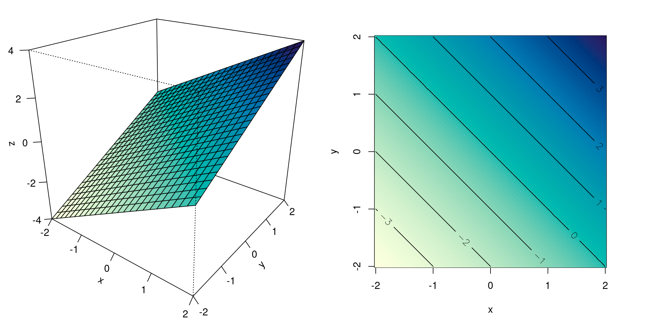
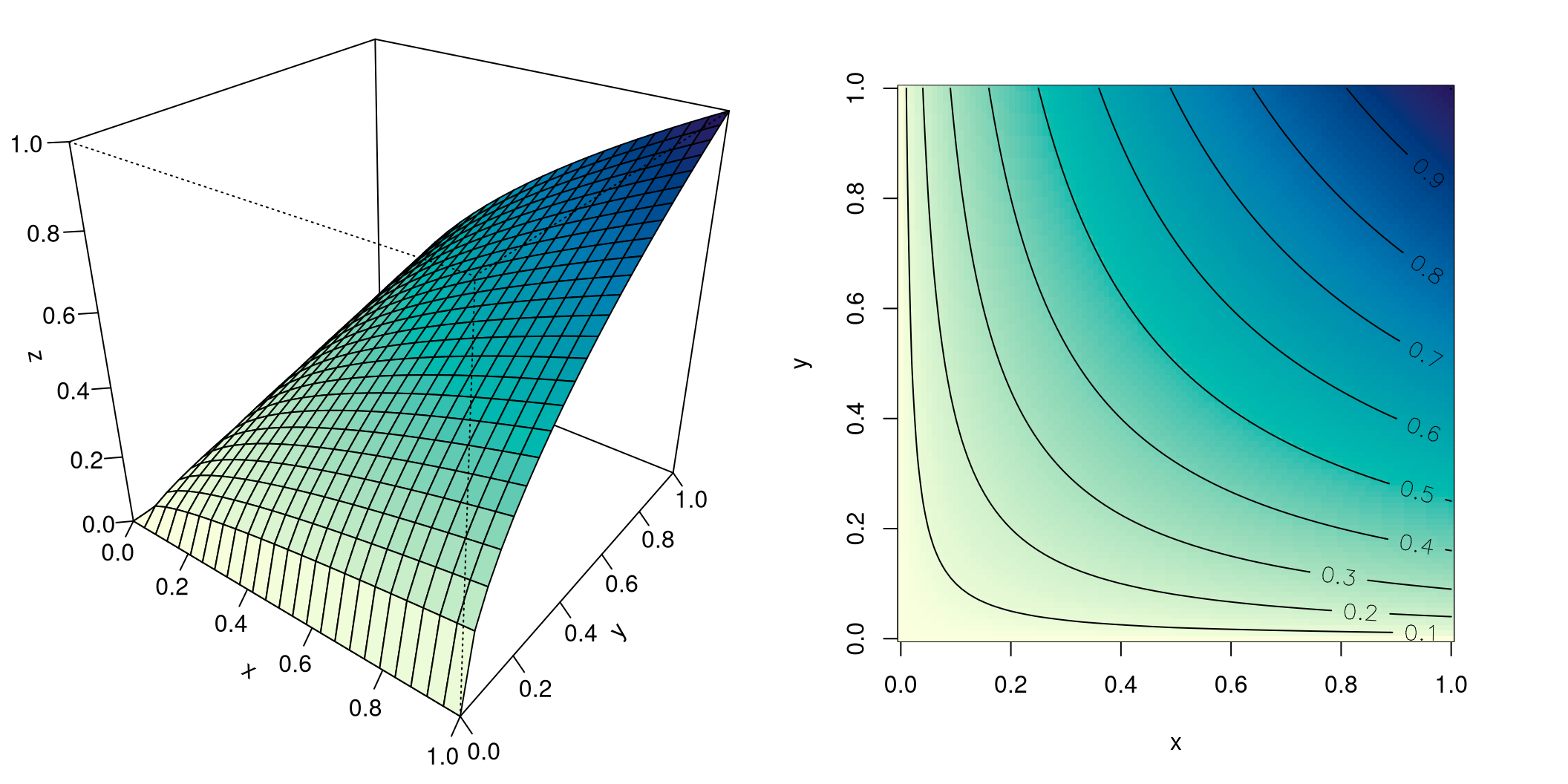
Figure 8.4 shows the linear function \(f(x,y) = x + y\). On the left, you see a perspective representation, the image of a tilted plane in space that contains the origin \(\boldsymbol{0}\).
On the right, you see the contour lines of this function: they are parallel lines running at equal distances. Each line is labeled with the value of the corresponding level.
Both the perspective representation and the contour lines are also superimposed with the same color gradient that encodes the levels of the function values in a similar way as in hiking maps: from bright yellow to dark blue for low to high function values.
The function term of a homogeneous linear function can be written as a matrix product: \[ \begin{gathered} f(x,y) = b_1x + b_2y = {\mathbf b}^\top \mathbf x, \quad \text{where } \mathbf x = \left(\begin{array}{c}x\\y\end{array}\right), \mathbf b = \left(\begin{array}{c}b_1\\b_2\end{array}\right). \end{gathered} \]
8.3.2 Quadratic Functions
Definition 8.5 A quadratic function with two variables is defined as a function with the function term \[ \begin{gathered} z = f(x,y) = a_{11}x^2 + 2a_{12}xy + a_{22}y^2 + b_1x + b_2y + c. \end{gathered} \] If \(b_1 = b_2 = c = 0\), then we call \[ \begin{gathered} f(x,y) = a_{11}x^2 + 2a_{12}xy + a_{22}y^2 \end{gathered} \] a homogeneous quadratic function.
The maximum domain of a quadratic function term is \(\mathbb R^2\).
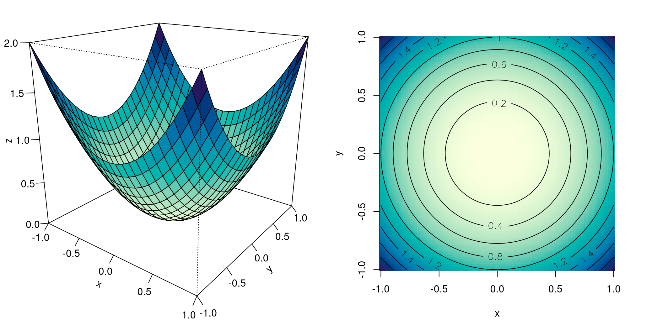
Figure 8.5 shows the homogeneous quadratic function \(f(x,y) = x^2 + y^2\). The perspective depiction shows a convex surface. The contour lines are of interest: they are concentric circles, with distances becoming ever smaller. We see why: the graph of the function becomes steeper the further we move from its minimum point, in any direction.
Now let’s make a minimal change to the example just shown, only one sign will be different. Now we are looking at the quadratic function \(f(x,y) = x^2 - y^2\):
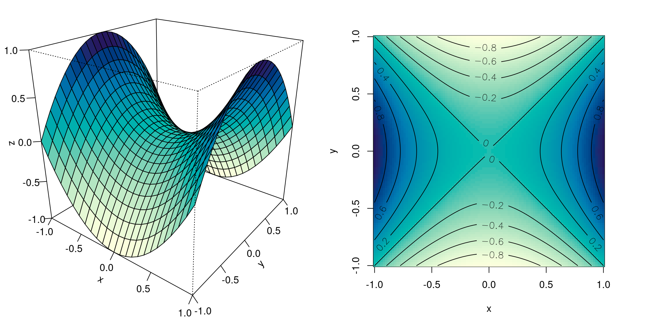
It reveals an entirely different picture! The perspective depiction shows a saddle surface, and the contour lines are concentric hyperbolas. They also show that they converge closer, and in four directions no less. Those are the directions in which the surface steeply ascends or descends.
Homogeneous quadratic functions will play an important role in our work, so let’s also consider how to represent them as matrix products. This is quite straightforward, but due to the quadratic terms, two matrix multiplications are necessary: \[ \begin{aligned} f(x,y) &= a_{11}x^2 + 2a_{12}xy + a_{22}y^2\\[5pt] &= (x,y)\left(\begin{array}{cc}a_{11} & \cellcolor{lgray}a_{12}\\ \cellcolor{lgray}a_{12} & a_{22}\end{array}\right) \left(\begin{array}{c}x\\y\end{array}\right) = {\mathbf x}^\top \mathbf A \mathbf x. \end{aligned} \] The matrix \(\mathbf A\) is called the generating matrix and we assume that this matrix is symmetric, meaning \({\mathbf A}^\top = \mathbf A\). This assumption is not necessary, but sensible in regard to the applications that we have in mind.
It is important to note that it is never necessary to carry out the matrix multiplications. Given the matrix \(\mathbf A\), we can directly read the quadratic function. The numbers in the main diagonal are the coefficients of \(x^2\) and \(y^2\), the sum of the off-diagonal components is the coefficient of \(xy\).
Exercise 8.6 Which homogeneous quadratic function is generated by the matrix \[ \begin{gathered} \mathbf A = \left(\begin{array}{rr}-2 & 5 \\5 & 8\end{array}\right) \end{gathered} \]
Solution: \(f(x,y) = -2x^2 + 10xy + 8y^2\). □
The reverse process is also very simple, that is, finding the generating matrix for a given function term.
We simply compare coefficients: the coefficient of \(x^2\) is \(a_{11}\), that of \(y^2\) is \(a_{22}\), finally, \(2a_{12}\) is the coefficient of \(xy\).
Exercise 8.7 Determine the matrix representation of the homogeneous quadratic functions:
-
\(f(x,y) = 2x^2 - 4xy + y^2\),
-
\(f(x,y) = x^2 - 3y^2\),
- \(f(x,y) = -6xy\).
Solution: We solve the task by coefficient comparison.
(a) \(2x^2\implies a_{11}=2\), \(y^2\implies a_{22}=1\), \(-4xy \implies a_{12}=-2\), thus the generating matrix is: \[ \begin{gathered} \mathbf A=\left(\begin{array}{rr}2 & -2\\-2 & 1\end{array}\right). \end{gathered} \]
In the same way, we find:
(b) \(\mathbf A=\left(\begin{array}{rr}1 & 0\\0 & -3\end{array}\right)\), (c) \(\mathbf A=\left(\begin{array}{rr}0 & -3\\-3 & 0\end{array}\right)\). □
Theorem 8.8 The general quadratic function has the matrix form: \[ \begin{gathered} f(\mathbf x)={\mathbf x}^\top \mathbf A \mathbf x+{\mathbf b}^\top \mathbf x+c,\qquad\text{where }{\mathbf A}^\top =\mathbf A\text{ and }\mathbf x=\left(\begin{array}{c}x\\y\end{array}\right). \end{gathered} \]
8.3.3 Cobb-Douglas Functions
In economic applications, so-called Cobb-Douglas functions play an important role.
Definition 8.9 A Cobb-Douglas function with two variables is understood as a function with the functional term \[ \begin{gathered} z=f(x,y)=Cx^{\alpha}y^{\beta}, \end{gathered} \] where \(\alpha\geq 0\) and \(\beta\geq 0\).
The maximal domain of a Cobb-Douglas function is usually \(\mathbb R_+^2\), the nonnegative quadrant.
Cobb-Douglas functions are often used as production functions. In this case, \(x\) and \(y\) describe the factor inputs, such as quantities of raw materials, energy, etc. The function value \(f(x,y)\) is the output given the factor input \(x\) and \(y\). In a macroeconomic context, \(x\) could represent the amount of total capital stock, \(y\) the national wage sum, \(f(x,y)\) the GDP. The level curves of the Cobb-Douglas function are curves of equal outputs, they are called isoquants.
8.3.4 Homogeneous Functions
While we have indicated homogeneous variants for linear and quadratic functions, this was not done for Cobb-Douglas functions. The reason is simple: Cobb-Douglas functions are inherently homogeneous.
We now clarify the concept of homogeneity:
Definition 8.10 A function \(f(x,y)\) is called homogeneous of degree \(k\), if for all \(t>0\): \[ \begin{gathered} f(tx,ty)=t^kf(x,y), \qquad k\in \mathbb R. \end{gathered} \tag{8.3}\]
The property of homogeneity is especially (but not only) of interest when \(f(x,y)\) is a production function. Now \(x\) and \(y\) are the amounts employed of two factors of production. If these amounts are doubled, i.e., \(t=2\), then the output changes by the factor \(2^k\). If \(k=1\), this means that doubling the input leads to doubling the output, one says also, the production function \(f(x,y)\) has constant returns to scale.
If \(k<1\), then \(f(x,y)\) has decreasing returns to scale; if \(k>1\), then the returns to scale are increasing.
A Cobb-Douglas function is homogeneous of degree \(\alpha+\beta\), for: \[ \begin{gathered} f(tx,ty)=C(tx)^\alpha(ty)^\beta=Ct^\alpha x^\alpha t^\beta y^\beta= Ct^{\alpha+\beta}x^\alpha y^\beta=t^{\alpha+\beta}f(x,y) \end{gathered} \]
8.4 The First Derivative
8.4.1 The Directional Derivative
In Chapter 3 we defined the first derivative of a function \(f(x)\) at a point \(x_0\) as the rate of change of the function at that point. But now our point \(\mathbf x=\mathbf a\) is an element of \(\mathbb R^2\), and at this point the change behavior of the function \(f(\mathbf a)\) will depend on which direction \(\mathbf v\) we look from \(\mathbf a\).
To be concrete about the direction, let us imagine a uniform motion in the plane \(\mathbb R^2\). It passes through the point \(\mathbf a\) and follows the displacement vector \(\mathbf v\ne \boldsymbol{0}\). In other words: \[ \begin{gathered} \mathbf x=\mathbf a+t\mathbf v\Leftrightarrow \left\{\begin{array}{ccc} x&=&a_1+tv_1\\ y&=&a_2+tv_2 \end{array} \right.,\qquad t\in\mathbb R \end{gathered} \] For each parameter value \(t\in\mathbb R\) we calculate \(\mathbf x=\mathbf a+t\mathbf v\) and the corresponding function value \(f(\mathbf x)\). This gives us a function \[ \begin{gathered} c(t)=f(\mathbf a+t\mathbf v)=f(a_1+tv_1,a_2+tv_2). \end{gathered} \] This function describes the function values of \(f\) along the uniform motion \(\mathbf x=\mathbf a+t\mathbf v\). And, importantly: \(c(t)\) is a function of only one variable \(t\)!
We are now interested in the rates of change of the function \(c(t)\). For this purpose, we calculate the derivative \(c'(t)\).
Before we name the child, let us consider a concrete example.
Let \(f(x,y)=3-x^2-y^2\), and let \(\mathbf x\) follow the uniform motion: \[ \begin{gathered} \mathbf x=\left(\begin{array}{c}-1\\-2\end{array}\right)+t\left( \begin{array}{r}1\\1\end{array}\right) \quad\Leftrightarrow\quad \left\{\begin{array}{ccl} x&=&-1 + t\\ y&=&-2 + t \end{array} \right. \end{gathered} \] We now substitute \(x\) and \(y\) into \(f(x,y)\) and obtain: \[ \begin{aligned} c(t)&=3-(-1 + t)^2-(-2 + t)^2\\ &=-2+6t-2t^2, \end{aligned} \] with first derivative: \[ \begin{gathered} c'(t)=6-4t. \end{gathered} \]
The functions from Example 8.11 are shown in Figure 8.8.
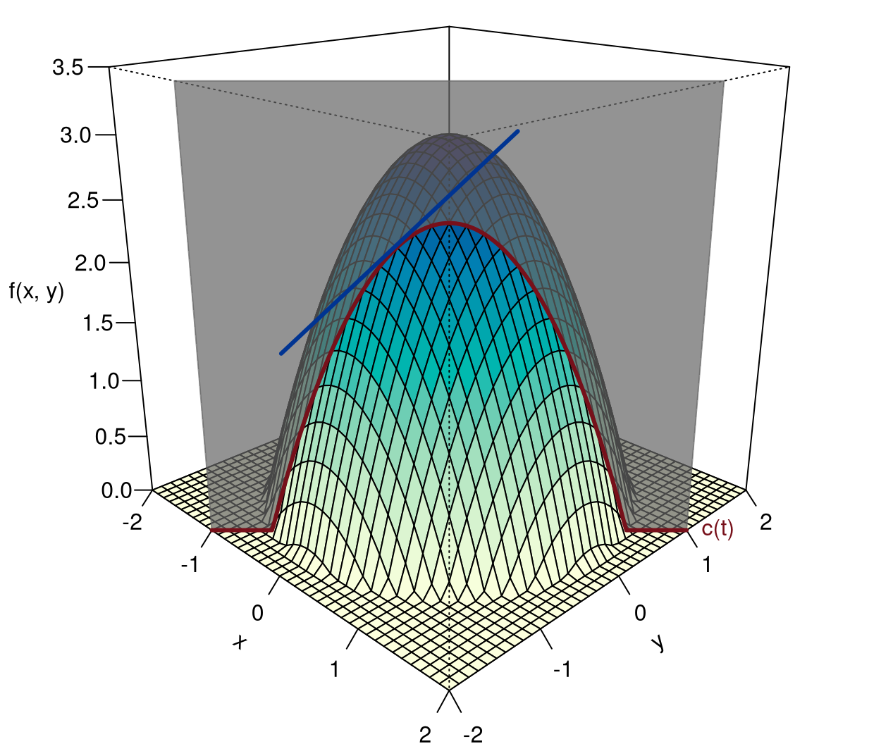
What we have just done is best illustrated thus: with a virtual knife, we make a cut perpendicular to the \((x,y)\)-plane through the mountain of functions. In doing so, we ensure:
- the cut goes through the point \(\mathbf a\), and
- has the direction \(\mathbf v\).
This creates a cut surface with a border, which is precisely the function \(c(t)\). If \(c(t)\) is differentiable, we can form its derivative \(c'(t)\). Its value at the position \(t=0\) is called the directional derivative at the point \(\mathbf x=\mathbf a\).
Definition 8.12 Let \(f(x,y)\) be a function in two variables and \(\mathbf x=\mathbf a+t\mathbf v\). If the function \[ \begin{gathered} c(t)=f(a_1+tv_1,a_2+tv_2) \end{gathered} \] has a first derivative at \(t=0\), then \(c'(0)\) is called the directional derivative of \(f(x,y)\) at the point \(\mathbf x=\mathbf a\). It indicates the rate of change of \(f(x,y)\) at the point \(\mathbf a\) in the direction of \(\mathbf v\).
Exercise 8.13 Determine the directional derivative of \(f(x,y)=xe^y\) at the point \(\mathbf a=\left(\begin{array}{r}-1\\1\end{array}\right)\) in the direction of \(\mathbf v=\left(\begin{array}{r}2\\-3\end{array}\right)\).
Solution: From the uniform motion \(\mathbf x=\mathbf a+t\mathbf v\) we get: \[ \begin{gathered} x=-1+2t,\quad y=1-3t. \end{gathered} \] Substitution into \(f(x,y)\) yields: \[ \begin{aligned} c(t)&=(-1+2t)e^{1-3t},\\[4pt] c'(t)&=2e^{1-3t}-3(-1+2t)e^{1-3t}=(5-6t)e^{1-3t},\\[4pt] c'(0)&=5e\simeq 13.59\,. \end{aligned} \] □
8.4.2 First Order Partial Derivatives
When we align the vector \(\mathbf v\) in the direction derivative parallel to the \(x\)- or \(y\)-axis, we obtain the first order partial derivatives of \(f(x,y)\).
Definition 8.14 (Partial Derivative) A partial derivative of a function \(f(x,y)\) with two variables is the derivative of the function \(f\) with respect to one of the two variables \(x\) or \(y\), while treating the other variable as a constant.
When we differentiate parallel to the \(x\)-axis, then \(\mathbf v=\left(\begin{array}{c}1\\0\end{array}\right)\). We call this the first partial derivative with respect to \(x\) and write it as \[ \begin{gathered} f_1'(x,y)\quad\text{or}\quad \frac{\partial f}{\partial x}. \end{gathered} \] Computationally, we obtain this derivative by treating \(y\) as a constant. Geometrically: we cut vertically parallel to the \(x\)-axis and differentiate the resulting edge, see Figure 8.9 left.
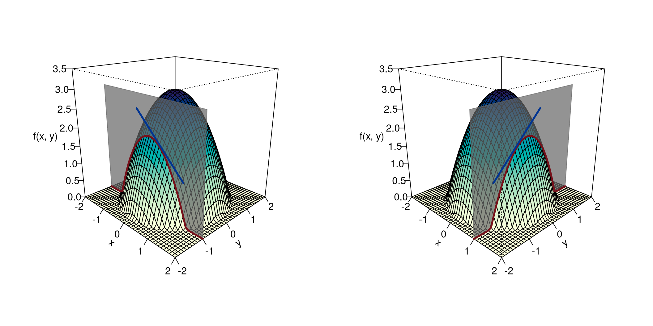
On the other hand, when we differentiate parallel to the \(y\)-axis, then \(\mathbf v=\left(\begin{array}{c}0\\1\end{array}\right)\). We call this the first partial derivative with respect to \(y\) and write it as \[ \begin{gathered} f_2'(x,y)\quad\text{or}\quad \frac{\partial f}{\partial y}. \end{gathered} \] Now \(x\) is treated as a constant, i.e., we cut vertically parallel to the \(y\)-axis and differentiate the resulting edge, see Figure 8.9 right.
Definition 8.15 We call the column vector of the first partial derivatives \[ \begin{gathered} \boldsymbol{f}'(\mathbf x)=\frac{\partial f}{\partial \mathbf x}=\left( \begin{array}{c} \frac{\partial f}{\partial x}\\[4pt] \frac{\partial f}{\partial y} \end{array}\right) \end{gathered} \] the first derivative or the gradient of \(f\).
Exercise 8.16 Find the first partial derivatives of the function \(f(x,y)=3x^2+e^{2y}\) at the point \(x=-1\) and \(y=0\).
Solution: First we differentiate partially with respect to \(x\). This means that \(y\) must be treated as a constant. It can occur as:
- A constant factor in a product, then it remains unchanged;
- Or as an additive constant. This becomes zero when differentiating.
If \(y\) is constant, then so is \(e^{2y}\), which appears as an additive constant in \(f(x,y)\). Therefore, the derivative of this term with respect to \(x\) is zero. Consequently \[ \begin{gathered} f_1'(x,y)=\frac{\partial f}{\partial x}=6x+0=6x,\\[4pt] f_1'(-1,0)=-6. \end{gathered} \] On the other hand, when we differentiate partially with respect to \(y\), \(x\) must be treated as a constant. Now the derivative of \(e^{2y}\) with respect to \(y\) is given by \(2e^{2y}\), while the term \(3x^2\) is an additive constant with respect to \(y\). Thus: \[ \begin{gathered} f_2'(x,y)=\frac{\partial f}{\partial y} =0+2e^{2y}=2e^{2y},\\[4pt] f_2'(-1,0)=2. \end{gathered} \] □
Exercise 8.17 Find the first partial derivatives of the function \(f(x,y)=3x^2e^{2y}\) at the point \(x=-1\) and \(y=0\).
Solution: When we differentiate partially with respect to \(x\), \(e^{2y}\) is a constant factor and as such is preserved: \[ \begin{aligned} f_1'(x,y)&=6xe^{2y},\qquad f_1'(-1,0)=-6. \end{aligned} \] On the other hand, if we differentiate with respect to \(y\), then \(3x^2\) is a constant factor: \[ \begin{gathered} f_2'(x,y)=3x^2\cdot 2e^{2y}=6x^2e^{2y},\qquad f_2'(-1,0)=6. \end{gathered} \] □
Exercise 8.18 Find the first partial derivatives of the function \(f(x,y)=\ln(2x-5y)\) at the point \(x=3\) and \(y=1\).
Solution: Here we need to use the Chain Rule for the logarithm (see Theorem 3.32). When differentiating with respect to \(x\), \(-5y\) is an additive constant within the inner function of the logarithm: \[ \begin{aligned} f_1'(x,y)&=\frac{2}{2x-5y}\qquad \text{(2 is the inner derivative: $(2x)'=2$)},\\[4pt] f_1'(3,1)&=2. \end{aligned} \] Similarly: \[ \begin{aligned} f_2'(x,y)&=-\frac{5}{2x-5y}\qquad \text{($-5$ is the inner derivative: $(-5y)'=-5$)},\\[4pt] f_2'(3,1)&=-5. \end{aligned} \] □
Exercise 8.19 Find the first partial derivatives of the function \(f(x,y)=5x^2e^{x-y^2}\) at the point \(x=1\) and \(y=0\).
Solution: When forming the first derivative with respect to \(x\), we have to use the Product Rule: \[ \begin{gathered} f_1'(x,y)=10xe^{x-y^2}+5x^2e^{x-y^2}=5x(2+x)e^{x-y^2},\\[5pt] f_1'(1,0)=15e\simeq 40.7742\,. \end{gathered} \] Now the derivative with respect to \(y\) (here we need the Chain Rule): \[ \begin{gathered} f_2'(x,y)=5x^2(-2y)e^{x-y^2}=-10x^2ye^{x-y^2},\\[5pt] f_2'(1,0)=0. \end{gathered} \] □
8.4.3 Derivative of Linear and Quadratic Functions
A linear function in one variable, i.e., \(y=bx+c\) has the first derivative \(y'=b\). Similarly, for linear functions in two variables: \[ \begin{aligned} f(\mathbf x)&={\mathbf b}^\top \mathbf x+c=b_1x+b_2y+c,\\[5pt] \left. \begin{array}{rcl}f_1'(\mathbf x)&=&b_1\\[5pt] f_2'(\mathbf x)&=&b_2\end{array} \right\}&\implies\boldsymbol{f}'(\mathbf x)=\mathbf b. \end{aligned} \] A general quadratic function in one variable is of the form \(y=ax^2+bx+c\) with the first derivative \(y'=2ax+b\). The same applies to quadratic functions in two variables!
In Theorem 8.8, the matrix form of a general quadratic function was given: \[ \begin{gathered} f(\mathbf x)={\mathbf x}^\top \mathbf A \mathbf x+{\mathbf b}^\top \mathbf x+c. \end{gathered} \] What is its first derivative? We start with the homogeneous term: \[ \begin{aligned} & {\mathbf x}^\top \mathbf A \mathbf x =a_{11}x^2+2a_{12}xy+a_{22}y^2\\[5pt] &\left.\begin{array}{rcl} \frac{\partial}{\partial x}{\mathbf x}^\top \mathbf A \mathbf x &\!=\!&2a_{11}x+2a_{12}y\\[5pt] \frac{\partial}{\partial y}{\mathbf x}^\top \mathbf A \mathbf x &\!=\!&2a_{12}x+2a_{22}y \end{array}\right\}\!\implies\\ & \frac{\partial}{\partial\mathbf x} {\mathbf x}^\top \mathbf A \mathbf x\!=\! 2\left(\!\begin{array}{cc}a_{11} & a_{12}\\a_{12} & a_{22}\end{array} \!\right)\left(\begin{array}{c}x\\y\end{array}\right)\!=\! 2\mathbf A\mathbf x \end{aligned} \] Now let’s put it all together:
Theorem 8.20 (Derivative of a Quadratic Function) Let \[ \begin{gathered} f(\mathbf x)={\mathbf x}^\top \mathbf A \mathbf x+{\mathbf b}^\top \mathbf x+c \end{gathered} \] be a general quadratic function. Then its first derivative is: \[ \begin{gathered} \boldsymbol{f}'(\mathbf x)=2\mathbf A\mathbf x+\mathbf b. \end{gathered} \]
8.4.4 Partial Rates of Change and Elasticities
The partial derivatives \(f_1'(x,y)\) and \(f_2'(x,y)\) measure the rate of change of \(f(x,y)\) in the direction of the \(x-\)axis and the \(y-\)axis, respectively, when the other variable is held constant. Analogously to the case of one variable, which was addressed in Chapter 3, for functions of two variables we can define partial elasticities as measures of responsiveness. They are derived as the partial derivative of the logarithm (relative rate of change) multiplied by \(x\) or \(y\):
Definition 8.21 Let \(f(x,y)>0\) be a function that is partially differentiable with respect to \(x\) and \(y\), then one calls \[ \begin{aligned} \epsilon_1(x,y)&=\frac{f_1'(x,y)}{f(x,y)}\cdot x=\frac{\partial\ln f(x,y)}{\partial x}\cdot x,\\[5pt] \epsilon_2(x,y)&=\frac{f_2'(x,y)}{f(x,y)}\cdot y=\frac{\partial\ln f(x,y)}{\partial y}\cdot y, \end{aligned} \tag{8.4}\] partial elasticities with respect to \(x\) and \(y\).
The elasticity \(\epsilon_1(x,y)\) tells us by what percentage \(f(x,y)\) changes with a small percentage change in \(x\), when \(y\) is held constant. \(\epsilon_2(x,y)\) is interpreted analogously.
Exercise 8.22 Let \(f(x,y)=100x^{0.3}y^{0.7}\) be a production function, with \(x\) and \(y\) representing the quantities of two factors of production, and \(f(x,y)\) the output produced. The task is to compute the partial production elasticities, i.e., the elasticities of \(f\) with respect to \(x\) and \(y\).
Solution: This is a linearly homogeneous Cobb-Douglas function, for which the partial production elasticities have a particularly simple form. We need the logarithmic derivatives, so we first form: \[ \begin{gathered} \ln f(x,y)=\ln\left(100x^{0.3}y^{0.7}\right)=\ln 100+0.3\ln x+0.7\ln y. \end{gathered} \] The logarithmic derivatives are: \[ \begin{gathered} \frac{\partial \ln f(x,y)}{\partial x}=\frac{0.3}{x},\qquad \frac{\partial \ln f(x,y)}{\partial y}=\frac{0.7}{y}. \end{gathered} \] From (8.4) it now follows: \[ \begin{gathered} \epsilon_1(x,y)=\frac{0.3}{x}\cdot x=0.3,\qquad \epsilon_2(x,y)=\frac{0.7}{y}\cdot y=0.7\,. \end{gathered} \] We see, that these elasticities are constant and independent of the factor input. Furthermore, they correspond to the exponents in \(f(x,y)\).
In general, for a Cobb-Douglas function \(f(x,y)=Cx^\alpha y^\beta\): \[ \begin{gathered} \epsilon_1(x,y)=\alpha,\qquad \epsilon_2(x,y)=\beta. \end{gathered} \] This is an important generalization of Theorem 3.54.
Remark 8.23 (Cross-Price Elasticity) It happens that the demanded quantity \(q\) of a good \(Q\) depends not only on its price \(p_1\) but also on the price \(p_2\) of a competing good \(R\). The demand function for \(Q\) then has the form of a function in two variables \(q:=q(p_1,p_2)\).
Cross-price elasticity is denoted as \(\epsilon_2(p_1,p_2)\). It measures how strongly the demand for \(Q\) reacts when the price of the competing product \(R\) changes. If \(\epsilon_2(p_1,p_2)>0\), this means that if the competing product \(R\) becomes more expensive, consumers switch and consume more of \(Q\). One also says that the two goods are substitutive or supplementary, such as energy from hydropower and nuclear power. Conversely, if \(\epsilon_2(p_1,p_2)<0\), an increasing price of \(R\) leads to less demand for both goods \(Q\) and \(R\). The two goods are complementary, like for example coffee machines and coffee capsules.
Exercise 8.24 The demanded quantity \(q\) of a good \(Q\) depends not only on its price \(p_1\) but also on the price \(p_2\) of a competing product \(R\). The demand function is: \[ \begin{gathered} q(p_1,p_2)=400-4p_1+3p_2. \end{gathered} \] To calculate are the partial price elasticities for current prices \(p_1=50\) and \(p_2=30\).
Solution: Here logarithmizing does not help much, so that we apply the first variant of (8.4): \[ \begin{aligned} \epsilon_1(p_1,p_2)&=\frac{q_1'(p_1,p_2)}{q(p_1,p_2)}\cdot p_1 =-\frac{4p_1}{400-4p_1+3p_2},\\[5pt] \epsilon_1(50,30)&=-\frac{200}{290}\approx -0.69\,. \end{aligned} \] An increase in the price \(p_1\) by 1% would cause a decrease in demand by approximately 0.69%, provided the price \(p_2\) remains unchanged.
Now the cross-price elasticity: \[ \begin{aligned} \epsilon_2(p_1,p_2)&=\frac{q_2'(p_1,p_2)}{q(p_1,p_2)}\cdot p_2 =\frac{3p_2}{400-4p_1+3p_2},\\[5pt] \epsilon_2(50,30)&=\frac{90}{290}\approx 0.31\,.\end{aligned} \] Thus, the two goods are substitutive. □
8.4.5 A First Variant of the Chain Rule
We have developed the concept of partial derivatives of a function in two variables using the idea of the directional derivative. This was simply done by specializing the displacement vector \(\mathbf v\) by aligning it parallel to one of the coordinate axes.
But can we also go the other way around? Can we determine the directional derivative for any \(\mathbf v\) given the known first partial derivatives \(\boldsymbol{f}'(\mathbf x)\)?
The answer is provided by the following theorem, which we will not prove:
Theorem 8.25 Let \(f\) be a function with two variables, having continuous partial derivatives. Furthermore, let \(\mathbf x=\mathbf a+t\mathbf v\) be a uniform motion and \(c(t)=f(\mathbf a+t\mathbf v)\) be the progression of the function \(f\) along this uniform motion. The first derivative \(c'(0)\) is given by: \[ \begin{gathered} c'(0)= f'_1(\mathbf a)v_1+f'_2(\mathbf a)v_2={\mathbf v}^\top \cdot \boldsymbol{f}'(\mathbf a). \end{gathered} \] This is the matrix product of the transpose of the displacement vector with the gradient.
Please note that this theorem explicitly provides the derivative of \(c(t)\) for \(t=0\), i.e., at the point \(\mathbf x=\mathbf a\).
In the following example, we investigate an interesting application of Theorem 8.25.
So far, we have always assumed that the demand for a good depends only on its price, possibly on the prices of competing products. But especially with durable consumer goods, the demand also depends on the income: the higher the income, the greater is the demand for certain goods.
Exercise 8.26 The demanded quantity \(q\) of a durable consumer good depends on income \(m\) and price \(p\) in the following manner: \[ \begin{gathered} q(m,p)=\frac{0.2m^2}{10+3p}. \end{gathered} \] Statistical studies have shown that both \(m\) and \(p\) increase linearly over time as follows: \[ \begin{gathered} \begin{array}{rcl} m(t)&=&1000+0.1t\\ p(t)&=&500+0.04t \end{array},\qquad t\ge 0\quad\text{(in years)}. \end{gathered} \] The current (\(t=0)\) rate of change in demand as a function of time is to be calculated.
Solution: The demand is a function of time: \[ \begin{gathered} c(t)=q(m(t),p(t))=\frac{0.2(1000+0.1t)^2}{10+3(500+0.04t)}. \end{gathered} \] To calculate \(c'(0)\), we apply Theorem 8.25. The linear growth of price and income causes a uniform motion in the \((m,p)\) plane: \[ \begin{gathered} \left(\begin{array}{c} m(t)\\ p(t) \end{array} \right)=\left(\begin{array}{c}1000\\500\end{array}\right)+t\left(\begin{array}{r}0.1\\0.04 \end{array}\right). \end{gathered} \] The displacement vector is \({\mathbf v}^\top =(0.1,0.04)\). Now we also need the vector of the first partial derivatives, the gradient of the function \(q(m,t)\), as well as the values of these derivatives for \(t=0\), i.e. for \(m=1000\) and \(p=500\): \[ \begin{gathered} \begin{array}{rclcrcl} q_1'(m,p)&=&\dfrac{0.4m}{10+3p} && q_1'(1000,500)&=&0.2649,\\[10pt] q_2'(m,p)&=&-\dfrac{0.6m^2}{(10+3p)^2} &&q_2'(1000,500)&=&-0.2631. \end{array} \end{gathered} \] Therefore, the instantaneous rate of change in demand is: \[ \begin{gathered} c'(0)=(0.1,0.04)\left(\begin{array}{r}0.2649\\-0.2631 \end{array} \right)=0.0160\,. \end{gathered} \] □
8.5 Second-Order Partial Derivatives
All previous examples have shown that the first partial derivatives of a function \(f(x,y)\) themselves are functions of \(x\) and \(y\). Therefore, we can try to differentiate each of these derivatives again with respect to \(x\) and \(y\) partially. There are four possible ways to form these second-order partial derivatives. The notation becomes a bit more complicated. We write: \[ \begin{gathered} \begin{array}{ll} f_{11}''(x,y)=\dfrac{\partial}{\partial x}\left(\dfrac{\partial f}{\partial x}\right)=\dfrac{\partial^2f}{\partial x^2}& f_{12}''(x,y)=\dfrac{\partial}{\partial x}\left(\dfrac{\partial f}{\partial y}\right)=\dfrac{\partial^2f}{\partial x\partial y}\\[12pt] f_{21}''(x,y)=\dfrac{\partial}{\partial y}\left(\dfrac{\partial f}{\partial x}\right)=\dfrac{\partial^2f}{\partial y\partial x}& f_{22}''(x,y)=\dfrac{\partial}{\partial y}\left(\dfrac{\partial f}{\partial y}\right)=\dfrac{\partial^2f}{\partial y^2} \end{array} \end{gathered} \] A word about the notation: \[ \begin{gathered} \frac{\partial}{\partial x}\quad\text{or}\quad \frac{\partial}{\partial y} \end{gathered} \] is called a differential operator. It means the command to partially differentiate, with respect to \(x\) or \(y\), whatever this operator is applied to.
The symbol \(f_{11}''(x,y)\) means: differentiate the first derivative with respect to \(x\), i.e., \(f_1'(x,y)\), again with respect to \(x\). This is particularly clear in operator notation.
Similarly: \(f_{22}''(x,y)\) means to differentiate \(f(x,y)\) partially with respect to \(y\) twice in a row.
The other two symbols indicate mixed derivatives.
\(f_{12}''(x,y)\) means: differentiate \(f(x,y)\) first with respect to \(y\) and then with respect to \(x\). With \(f_{21}''(x,y)\), it is the other way around.
Thus, there are four second-order derivatives, but in most cases we only need to calculate three because if the mixed derivatives are continuous, then they are equal, that is, \(f_{12}''(x,y)=f_{21}''(x,y)\). Therefore, the order of differentiation does not matter.
Similar to how we combined the first derivatives into a vector, the gradient, we combine the second derivatives into a matrix, the Hessian matrix of the function \(f(x,y)\): \[ \begin{gathered} \boldsymbol{f}''(x,y)=\left(\begin{array}{cc} f_{11}''(x,y) & f_{12}''(x,y)\\ f_{21}''(x,y) & f_{22}''(x,y) \end{array} \right), \end{gathered} \] or we can also write equivalently: \[ \begin{gathered} \boldsymbol{f}''(\mathbf x)=\left(\begin{array}{cc} f_{11}''(\mathbf x) & f_{12}''(\mathbf x)\\ f_{21}''(\mathbf x) & f_{22}''(\mathbf x) \end{array} \right). \end{gathered} \]
Exercise 8.27 Determine the Hessian matrix of the function \(f(x,y)=2xy^3-y^2+5x-7\) at the point \({\mathbf a}^\top =(1,\,2)\).
Solution: First, we compute the first partial derivatives with respect to \(x\) and \(y\): \[ \begin{gathered} f_1'(x,y)=2y^3+5,\qquad f_2'(x,y)=6xy^2-2y. \end{gathered} \] Then, one after the other: \[ \begin{gathered} f_{11}''(x,y)=\frac{\partial}{\partial x}(2y^3+5)=0, \end{gathered} \] this must be zero because we are differentiating with respect to \(x\) and \(2y^3+5\) is therefore constant. \[ \begin{gathered} f_{22}''(x,y)=\frac{\partial}{\partial y}(6xy^2-2y)=12xy-2. \end{gathered} \] For the mixed derivatives, we get: \[ \begin{aligned} f_{12}''(x,y)&=\frac{\partial}{\partial x}(6xy^2-2y)=6y^2,\\[5pt] f_{21}''(x,y)&=\frac{\partial}{\partial y}(2y^3+5)=6y^2=f_{12}''(x,y). \end{aligned} \] Thus, we have the Hessian matrix: \[ \begin{gathered} \boldsymbol{f}''(x,y)=\left(\begin{array}{cc} 0 & 6y^2\\6y^2 &12xy-2 \end{array} \right),\qquad \boldsymbol{f}''(1,2)=\left(\begin{array}{cc} 0 & 24\\24 &22 \end{array} \right). \end{gathered} \] □
Exercise 8.28 We are looking for the Hessian matrix of \(f(x,y)=x/y\) at the point \({\mathbf a}^\top =(1,-1)\).
Solution: The first partial derivatives are: \[ \begin{gathered} f_1'(x,y)=\frac{1}{y},\qquad f_2'(x,y)=-\frac{x}{y^2}. \end{gathered} \] Further: \[ \begin{gathered} f_{11}''(x,y)=\frac{\partial}{\partial x}\frac{1}{y}=0,\quad f_{22}''(x,y)=\frac{\partial}{\partial y}\left(-\frac{x}{y^2}\right) = \frac{2x}{y^3}, \end{gathered} \] and \[ \begin{gathered} f_{12}''(x,y)=\frac{\partial}{\partial x}\left(-\frac{x}{y^2}\right) =-\frac{1}{y^2}=f_{21}''(x,y). \end{gathered} \] Therefore, the Hessian matrix is: \[ \begin{gathered} \boldsymbol{f}''(x,y)=\left(\begin{array}{rr} 0 & -\dfrac{1}{y^2}\\[10pt] -\dfrac{1}{y^2} & \dfrac{2x}{y^3} \end{array} \right),\qquad \boldsymbol{f}''(1,-1)=\left(\begin{array}{rr} 0 & -1\\-1 & -2 \end{array} \right). \end{gathered} \] □
8.5.1 The Second Derivative of a Quadratic Function
In deriving Theorem 8.20, we have already found out: if \(g(x,y)=a_{11}x^2+2a_{12}xy+a_{22}y^2\) is a homogeneous quadratic function, then: \[ \begin{gathered} \left. \begin{array}{rcl} g_1'(x,y)&=&2a_{11}x+2a_{12}y\\[5pt] g_2'(x,y)&=&2a_{12}x+2a_{22}y \end{array}\right\}\implies \boldsymbol{g}'(\mathbf x)=2\mathbf A\mathbf x.\qquad \mbox{(A)} \end{gathered} \] Now we form the second partial derivatives in (A): \[ \begin{gathered} \left. \begin{array}{rclcrcl} g_{11}''(x,y)&=&2a_{11} && g_{12}''(x,y)&=&2a_{12}\\[5pt] g_{21}''(x,y)&=&2a_{12} && g_{22}''(x,y)&=&2a_{22} \end{array}\right\}\implies \boldsymbol{g}''(\mathbf x)=2\mathbf A \end{gathered} \] This leads to the important result:
Theorem 8.29 (Second Derivative of a Quadratic Function) Let \[ \begin{gathered} f(\mathbf x)={\mathbf x}^\top \mathbf A \mathbf x+{\mathbf b}^\top \mathbf x+c \end{gathered} \] be a general quadratic function. Then its second derivative is: \[ \begin{gathered} \boldsymbol{f}''(\mathbf x)=2\mathbf A \end{gathered} \]
Notice the nice analogy to quadratic functions in one variable \(y=ax^2+bx+c\). Their second derivative is \(y''=2a\).
8.5.2 The Second Derivative in a Direction
The following result will prove to be extraordinarily important in our next venture, optimization of functions in two variables.
Once again, we consider a linear vertical cut \(c(t)\) along \(\mathbf x=\mathbf a+t\mathbf v, \mathbf v\ne \boldsymbol{0}\) through the function mountain range. Now we are interested in the value of the second derivative \(c''(0)\). If \(c'(0)=0\), then there is a critical point of the section curve \(c(t)\) at \(t=0\), i.e., at the point \(\mathbf x=\mathbf a\), and we know from Chapter 3 that we can make the decision about whether this critical point is a maximum or minimum based on the sign of the second derivative. The following theorem, in which the Hessian matrix plays a key role, is actually also a variant of the chain rule like Theorem 8.25.
Theorem 8.30 Let \(f\) be a function of two variables, with continuous second partial derivatives. Furthermore, let \(\mathbf x=\mathbf a+t\mathbf v\) be uniform motion and \(c(t)=f(\mathbf a+t\mathbf v)\). Then, the 2nd derivative of the section curve \(c(t)\) for \(t=0\), i.e., at the point \(\mathbf x=\mathbf a\), is: \[ \begin{aligned} c''(0)&= f''_{11}(\mathbf a)v_1^2+2f''_{12}(\mathbf a)v_1v_2+f''_{22}(\mathbf a)v_2^2\\[5pt] &= (v_1,v_2)\left(\begin{array}{cc} f_{11}''(\mathbf a) & f_{12}''(\mathbf a) \\[4pt] f_{21}''(\mathbf a) & f_{22}''(\mathbf a) \end{array} \right)\left(\begin{array}{c}v_1\\v_2\end{array}\right)={\mathbf v}^\top \boldsymbol{f}''(\mathbf a) \mathbf v. \end{aligned} \] This is the homogeneous quadratic function generated by the Hessian matrix at point \(\mathbf a\).
8.6 Global Optimization
In this section, we embark on the search for extremal values of a function \(f(x,y)\) with two variables. To recall, in Chapter 3 we stated the rule for functions in one variable:
Let \(x_0\) be a critical point of a function \(f(x)\), i.e. \(f'(x_0)=0\). This point is a relative maximum if \(f''(x_0)<0\), and a relative minimum if \(f''(x_0)>0\).
We will find that things are not fundamentally different for functions of two variables. However, our results will be more general than in Chapter 3, where we limited ourselves to relative, i.e. local extreme values. Now we are looking for global extremal points of a function.
8.6.1 Critical Points
Let \(f:M\to\mathbb R\), \(M\subseteq\mathbb R^2\), be a differentiable function of two variables.
A point \(\mathbf a\in M\) is a global maximum of \(f\) if \[ \begin{gathered} f(\mathbf x)\le f(\mathbf a)\quad\text{for all $\mathbf x\in M$}. \end{gathered} \] A point \(\mathbf a\in M\) is a global minimum of \(f\) if \[ \begin{gathered} f(\mathbf x)\ge f(\mathbf a)\quad\text{for all $\mathbf x\in M$}. \end{gathered} \] It is quite simple to state a condition (equation) that must be satisfied by any global maximum or global minimum.
Theorem 8.31 Let \(f\) be a function of two variables with a continuous derivative, and let \(\mathbf a\) be an interior point of \(M\).
If the point \(\mathbf a\) is a global maximum or a global minimum of \(f\), then \(\mathbf a\) must be a critical point of \(f\), which means the equation \[ \begin{gathered} f'(\mathbf a)=\boldsymbol{0} \end{gathered} \] must be satisfied.
In other words: At a global maximum or global minimum of a function, all first-order partial derivatives are equal to zero.
Reasoning: If \(\mathbf a\) is a global maximum of \(f\), then \(\mathbf a\) is also a maximum of \(f\) along uniform motion \(\mathbf x=\mathbf a+t\mathbf v\) with any arbitrary displacement vector \(\mathbf v\ne \boldsymbol{0}\). Hence, \(c(t)=f(\mathbf a+t\mathbf v)\) has a maximum at \(t=0\), and it follows from Theorem 8.25: \[ \begin{gathered} 0=c'(0)={\mathbf v}^\top \cdot \boldsymbol{f}'(\mathbf a)=f'_1(\mathbf a)v_1+f'_2(\mathbf a)v_2 \end{gathered} \] for any arbitrary displacement vector \(\mathbf v\ne \boldsymbol{0}\). But this is only possible if both partial derivatives \(f'_1(\mathbf a)\) and \(f'_2(\mathbf a)\) are zero.
A similar argument applies to a global minimum. □
Every optimum is thus a critical point and critical points can be found as solutions to equations.
8.6.2 Convex Functions
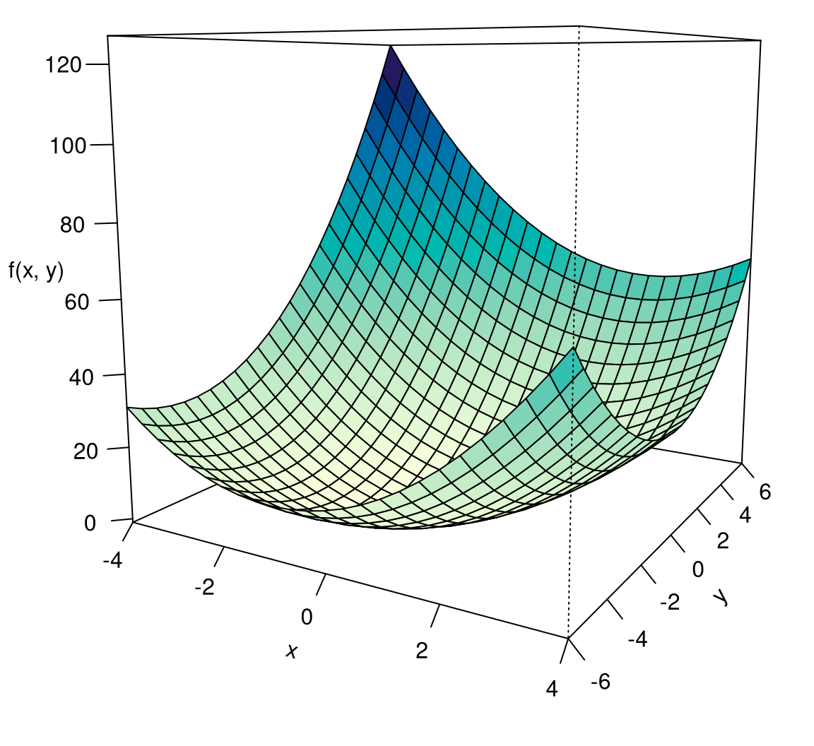
Exercise 8.32 Find a global minimum of the quadratic function \[ \begin{gathered} f(x,y)=2x^2-xy+y^2-2x+4y+3. \end{gathered} \] It is represented in Figure 8.10.
Solution: If the function has a global minimum at all, it must be a critical point. Therefore, we calculate the partial derivatives \[ \begin{gathered} f'_1(x,y)=4x-y-2,\quad f'_2(x,y)=-x+2y+4, \end{gathered} \] and solve the system of equations \(f'_1=0\), \(f'_2=0\), that is. \[ \begin{aligned} 4x-y-2&=0\\ -x+2y+4&=0 \end{aligned} \] The solution is \(x=0\), \(y=-2\), hence the only critical point of \(f(x,y)\) is the point \({\mathbf a}^\top =(0,-2)\).
Thus, if the function \(f(x,y)\) has a global minimum, then the point \(\mathbf a\) is the only candidate.
But how can we be sure that the point \(\mathbf a\) really is a global minimum?
For that purpose, we examine the second derivative of \(f\).
The Hessian matrix of \(f\) is: \[ \begin{gathered} \boldsymbol{f}''(x,y)=\left(\begin{array}{rr}4 & -1\\-1 & 2\end{array}\right). \end{gathered} \] Now we consider uniform movements in the \((x,y)\)-plane, all passing through the critical point \(\mathbf a\) and have an arbitrary displacement vector \(\mathbf v\ne \boldsymbol{0}\). In other words: we make vertical cuts through point \(\mathbf a\), the direction of every cut being \(\mathbf v\). Each of these cuts yields a boundary curve \(c(t)\).
If \(\mathbf a\) is actually a global minimum of \(f(x,y)\), then \(\mathbf a\) must not only be a critical point of every \(c(t)\) but it must also be a minimum on every \(c(t)\), meaning, \(c''(0)\ge 0\).
This can be evaluated with Theorem 8.30: it must hold for every \(\mathbf v\ne \boldsymbol{0}\): \[ \begin{gathered} {\mathbf v}^\top \boldsymbol{f}''(\mathbf a) \mathbf v={\mathbf v}^\top \left(\begin{array}{rr}4 & -1\\-1 & 2\end{array}\right) \mathbf v\ge 0. \end{gathered} \] Now we write (as described under Figure 8.6) this homogeneous quadratic function in more detail: \[ \begin{aligned} {\mathbf v}^\top \boldsymbol{f}''(\mathbf a) \mathbf v&=4v_1^2-2v_1v_2+2v_2^2\\[5pt] &=\underbrace{4v_1^2-2v_1v_2+\frac{1}{4}v_2^2}_{}\; \underbrace{-\frac{1}{4}v_2^2+2v_2^2}_{}\\[5pt] &=\left(2v_1-\frac{1}{2}v_2\right)^2+\frac{7}{4}v_2^2\ge 0, \end{aligned} \] Both terms (they are squares!) are non-negative, and therefore so is their sum.
The second derivative along any uniform movement is apparently always non-negative. Therefore, \(\mathbf a\) is a global minimum of \(f\) along every uniform movement through \(\mathbf a\), and thus is a global minimum in general. □
In this example, we have seen that for a function where all second derivatives along uniform movements \(\mathbf a+t\mathbf v\) are non-negative, any critical point \(\mathbf a\) must be a global minimum.
We now summarize everything, introducing important new concepts.
Definition 8.33 A symmetric matrix \(\mathbf A\) of order \(n\times n\) is called positive semidefinite when \({\mathbf v}^\top \mathbf A\mathbf v\ge 0\) for all \(\mathbf v\in\mathbb R^n\).
Definition 8.34 A function \(f\) with two variables and a continuous second derivative is called convex if its Hessian matrix is positive semidefinite everywhere.
The property of a function being convex means graphically that its graph is curved downwards. Figure 8.10 shows a convex function.
Theorem 8.35 In a convex function, every critical point is a global minimum.
So, with convex functions, it’s especially easy to find a global minimum: It suffices to find any critical point!
Whether a function \(f\) is convex can be determined by checking if its Hessian matrix is positive semidefinite. The following rule is helpful for this purpose.
Theorem 8.36 A symmetric \(2\times 2\) matrix \(\mathbf A= \left(\begin{array}{cc}a & b\\b & c\end{array}\right)\) is positive semidefinite if and only if \(a\ge 0\), \(c\ge 0\), and \(\det\mathbf A\ge 0\).
Justification: First, consider the case \(a\not=0\). We have \[ \begin{aligned} {\mathbf v}^\top \mathbf A\mathbf v&=av_1^2+2bv_1v_2+cv_2^2\\ &=a\Big(v_1+\frac{b}{a}v_2\Big)^2+\Big(c-\frac{b^2}{a}\Big)v^2_2. \end{aligned} \] This is \(\ge 0\) for all \(v_1,\,v_2\in\mathbb R\) if and only if \(a\ge 0\) and \(ac\ge b^2\). The latter condition implies \(c\ge 0\) and is also equivalent to \(\det \mathbf A\ge 0\).
On the other hand, if \(a=0\), then \[ \begin{gathered} {\mathbf v}^\top \mathbf A\mathbf v=2bv_1v_2+cv_2^2, \end{gathered} \] and this expression can only be \(\ge 0\) for all \(\mathbf v\ne \boldsymbol{0}\) if \(b=0\) and \(c\ge 0\). However, if \(a=0\) and \(b=0\), then \(\det\mathbf A=0\) as well. □
Convex functions have many remarkable properties. Among others, sums of convex functions are also convex. Therefore, the following holds:
Theorem 8.37 Linear functions \(g(x,y)={\mathbf b}^\top \mathbf x+c\) are convex, since their Hessian matrix is the zero matrix, which is positive semidefinite. If \(f(x,y)\) denotes a convex function of two variables, then \(f(x,y)+{\mathbf b}^\top \mathbf x+c\) is also convex.
8.6.3 Concave Functions
If a function \(f\) is convex, then \(-f\) is concave, meaning it is curved upwards. Everything we’ve discussed about convex functions applies mutatis mutandis to concave functions. We summarize:
Definition 8.38 A symmetric matrix \(\mathbf A\) of order \(n\times n\) is called negatively semidefinite, if \({\mathbf v}^\top \mathbf A\mathbf v\le 0\) for all \(\mathbf v\in\mathbb R^n\).
Definition 8.39 A function \(f\) with two variables and a continuous second derivative is concave if its Hessian matrix is negatively semidefinite everywhere.
Theorem 8.40 With a concave function, every critical point is a global maximum.
Thus, for concave functions, it is particularly easy to find a global maximum: just find any critical point!
To determine if a function \(f\) is concave, one must check whether its Hessian matrix is negatively semidefinite. The following rule is helpful in this regard.
Theorem 8.41 A symmetric \(2\times 2\)-matrix \(\mathbf A=\left(\begin{array}{cc}a & b\\b & c\end{array}\right)\) is negatively semidefinite if and only if \(a\le 0, c\le 0\) and \(\det \mathbf A\ge 0\).
Justification: In the case of \(a\ne 0\): \[ \begin{aligned} {\mathbf v}^\top \mathbf A\mathbf v&=av_1^2+2bv_1v_2+cv_2^2\\[5pt] &=a\Big(v_1+\frac{b}{a}v_2\Big)^2+\Big(c-\frac{b^2}{a}\Big)v^2_2 \end{aligned} \] This is \(\le 0\) for all \(v_1,\,v_2\in\mathbb R\) if \(a\le 0\) and \(c-\frac{b^2}{a}\le 0\), that is, \(ac\ge b^2\). The latter condition implies (since \(a\le 0\)) that \(c\le 0\) and is equivalent to \(\det \mathbf A\ge 0\).
The case of \(a=0\) can be shown analogously. □
Exercise 8.42 Find the optimum of the function \(f(x,y)=e^{-x^2-y^2}\).
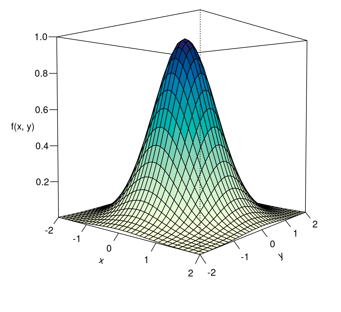
Solution: First, we embark on a search for a critical point. To do this, we form the first derivatives and set them to zero:
\[ \begin{gathered} f_1'(x,y)=-2xe^{-x^2-y^2},\quad f_2'(x,y)=-2ye^{-x^2-y^2}. \end{gathered} \] The conditions \(f_1'(x,y)=0\) and \(f_2'(x,y)=0\) are only met at the point \(x=0, y=0\), because the exponential function is always \(>0\). Therefore, there is a critical point at \({\mathbf a}^\top =(0,0)\).
Now we form the Hessian matrix, noting that we must apply the product rule for \(f_{11}''(x,y)\) and \(f_{22}''(x,y)\): \[ \begin{gathered} \begin{array}{ll} f_{11}''(x,y)=-2(1-2x^2)e^{-x^2-y^2} & f_{12}''(x,y)=4xye^{-x^2-y^2}\\[5pt] f_{21}''(x,y)= 4xye^{-x^2-y^2} & f_{22}''(x,y)=-2(1-2y^2)e^{-x^2-y^2} \end{array} \end{gathered} \] The Hessian matrix and its value at the critical point are therefore: \[ \begin{aligned} \boldsymbol{f}''(\mathbf x)&=e^{-x^2-y^2}\left(\begin{array}{cc} -2(1-2x^2) & 4xy\\4xy & -2(1-2y^2) \end{array} \right),\\ \boldsymbol{f}''(0,0)&=\left(\begin{array}{rr}-2 & 0\\0 & -2\end{array}\right). \end{aligned} \] However, the matrix \(\boldsymbol{f}''(0,0)\) is negative semidefinite, according to Theorem 8.41, as both its main diagonal components are negative and its determinant has the value \(4>0\). Therefore, the point \((0,0)\) is a global maximum. □
8.6.4 Quadratic Functions
For quadratic functions \[ \begin{gathered} f(\mathbf x)={\mathbf x}^\top \mathbf A\mathbf x+{\mathbf b}^\top \mathbf x+c,\qquad \mbox{(A)} \end{gathered} \] it is particularly easy to determine whether they are convex or concave. According to Theorem 8.29, their Hessian matrix is \(2\mathbf A\). We then simply apply Theorem 8.36 or Theorem 8.41.
If the matrix \(\mathbf A\) generating the homogenous part is regular, i.e., it has an inverse, then the optimum is even uniquely determined. Because when we differentiate (A) and set the first derivative to zero (see Theorem 8.20) we obtain: \[ \begin{gathered} \boldsymbol{f'}(\mathbf x)=2\mathbf A\mathbf x+\mathbf b=\boldsymbol{0}.\qquad \mbox{(B)} \end{gathered} \] We solve this matrix equation for \(\mathbf x\) (see Chapter 7): \[ \begin{gathered} \mathbf x=-\frac{1}{2}\mathbf A^{-1}\mathbf b. \end{gathered} \] If, on the other hand, \(\mathbf A\) is singular, then we must strive for the general solution of the linear equation system (B). If there is a solution at all, then we have infinitely many critical points and thus just as many optima!
Exercise 8.43 A monopoly company offers two goods at prices \(p_1\) and \(p_2\). Demand is determined by the demand functions \[ \begin{aligned} D_1(p_1,p_2):&\quad q_1=310-4p_1+p_2\\ D_2(p_1,p_2):&\quad q_2=248+p_1-8p_2 \end{aligned} \] The variable costs for producing the goods are 20 and 14 monetary units, respectively, and the fixed costs are 10,000 monetary units. At what prices should the goods be offered to maximize profit?
Solution: The profit is, as usual, the difference between revenues and costs: \[ \begin{aligned} \pi(p_1,p_2)&=p_1q_1+p_2q_2-20q_1-14q_2-10000\\[4pt] &=p_1(310-4p_1+p_2)+p_2(248+p_1-8p_2)-\\[4pt] &\qquad -20(310-4p_1+p_2)-14(248+p_1-8p_2)-10000\\[4pt] &=-4p_1^2+2p_1p_2-8p_2^2+376p_1+340p_2-19762 \end{aligned} \] This is a quadratic function \[ \begin{gathered} \pi(\mathbf p)={\mathbf p}^\top \mathbf A\mathbf p+{\mathbf b}^\top \mathbf p+c,\qquad {\mathbf p}^\top =(p_1,p_2), \end{gathered} \] with \[ \begin{gathered} \mathbf A=\left(\begin{array}{rr}-4 & 1\\ 1 & -8\end{array}\right), \quad\mathbf b=\left(\begin{array}{c}376\\340\end{array}\right),\quad c=-19672. \end{gathered} \] The Hessian matrix of \(\pi(\mathbf p)\) is: \[ \begin{gathered} \boldsymbol{\pi}''(\mathbf p)=2\mathbf A=\left( \begin{array}{rr}-8 & 2\\2 & -16\end{array}\right), \end{gathered} \] this is certainly negative semi-definite, because both principal diagonal components are negative and \(\det(2\mathbf A)=124\) is positive. Therefore, \(\pi(\mathbf p)\) is concave and every critical point is a global maximum.
In fact, there is only one maximum, because \(\det\mathbf A=31\ne 0\). \(\mathbf A\) therefore has an inverse and thus: \[ \begin{aligned} \mathbf p&=-\frac{1}{2}\mathbf A^{-1}\mathbf b\\[4pt] &=-\frac{1}{2}\,\frac{1}{31}\left(\begin{array}{rr}-8 & -1\\-1 & -4\end{array} \right)\left(\begin{array}{c}376\\340\end{array}\right) =\left(\begin{array}{c}54\\28\end{array}\right). \end{aligned} \] The pricing \(p_1=54, p_2=28\) guarantees maximum profit. □
8.7 Chain Rule and Implicit Functions
8.7.1 The Chain Rule
Let \(f:M\to\mathbb R\), \(M\subseteq\mathbb R^2\), be a function in two variables.
So far, we have examined the course of the function \(f(x,y)\) along a uniform motion \[ \begin{gathered} \mathbf x=\mathbf g(t)=\mathbf a+t\mathbf v,\;\text{that is:}\; \left\{ \begin{array}{l} x=g_1(t)=a_1+tv_1\\ y=g_2(t)=a_2+tv_2 \end{array} \right. \end{gathered} \] \(t\in\mathbb R\). Such a uniform movement is a vector-valued function \(\mathbf x=\mathbf g(t)\), whose both components \(g_1(t)\) and \(g_2(t)\) are linear functions of the parameter \(t\).
However, we sometimes want to examine the course of a function \(f\) along a non-linear function \(\mathbf x=\mathbf g(t)\). We call such a function \(\mathbf x=\mathbf g(t)\) a path. A uniform motion is therefore a special path that is first, straight and second, traversed with constant speed.
For each parameter value \(t\in\mathbb R\), we calculate the corresponding point \(\mathbf x=\mathbf g(t)\) and with it the function value \(f(\mathbf x)=f(x,y)\). This gives us a function \[ \begin{gathered} c(t)=f(\mathbf g(t))=f(g_1(t),g_2(t)),\qquad x=g_1(t),\;y=g_2(t). \end{gathered} \] This function describes the function values of \(f\) along the path \(\mathbf x=\mathbf g(t)\).
Exercise 8.44 A manufacturer produces a good from two raw materials \(A\) and \(B\), where the production function is given by \[ \begin{gathered} q=f(x,y)=200x^{0.7}y^{0.3} \end{gathered} \] This means that the use of \(x\) tons of raw material \(A\) and \(y\) tons of raw material \(B\) results in \(q=f(x,y)\) units of the final product.
At the moment, the manufacturer uses 20 tons of \(A\) and 15 tons of \(B\) per week. However, the supply of the raw material \(A\) decreases by 4 percent per week, while the supplied amount of the raw material \(B\) increases by 3 percent.
How will the produced quantities of the final product develop and what is the current rate of relative change?
Solution: The deliveries of raw materials \(A\) and \(B\) have constant relative change rates \(c_1=\ln 0.96=-0.0408\) and \(c_2=\ln 1.03=0.0296\). They are therefore described by the exponential functions \[ \begin{gathered} \mathbf x=\mathbf g(t)=\left\{ \begin{array}{l} g_1(t)=20\cdot 0.96^t=20e^{-0.0408 t}\\[5pt] g_2(t)=15\cdot 1.03^t=15e^{0.0296 t} \end{array} \right. \end{gathered} \] The vector-valued function \(\mathbf x=\mathbf g(t)\) is an example of a nonlinear path.
The produced quantity \(q=f(x,y)\) of the final product is obtained by inserting the path \(\mathbf x=\mathbf g(t)\) into the production function \(q=f(\mathbf x)\): \[ \begin{aligned} c(t)=f(g_1(t),g_2(t))&=200(20e^{-0.0408 t})^{0.7}(15e^{0.0296 t})^{0.3}\\[4pt] &=200\cdot 20^{0.7}\cdot e^{-0.0408\cdot 0.7t}\cdot 15^{0.3}\cdot e^{0.0296\cdot 0.3t}\\[4pt] &=3669.3 \,e^{-0.0197t}. \end{aligned} \] From this, the relative change rate follows \[ \begin{gathered} \frac{c'(t)}{c(t)}=-0.0197\;. \end{gathered} \] Therefore, production decreases weekly at a rate of \(1.97\) %. □
We can significantly simplify the calculation procedure of the last task.
Let \(\mathbf x=\mathbf g(t)\) be a differentiable path. Then we call \[ \begin{gathered} \mathbf g'(t)=\left(\begin{array}{c}g_1'(t)\\g_2'(t) \end{array}\right) \end{gathered} \] the velocity vector of this path. In the case of uniform motion \[ \begin{gathered} \mathbf g(t)=\mathbf x=\mathbf a+t\mathbf v=\left\{ \begin{array}{l} a_1+tv_1\\a_2+tv_2 \end{array}\right. \end{gathered} \] the velocity vector \(\mathbf g'(t)=\left(\begin{array}{c}v_1\\v_2 \end{array}\right)=\mathbf v\) is constant (it does not depend on the parameter \(t\)).
Exercise 8.45 Determine the velocity vector of \[ \begin{gathered} \mathbf x=\mathbf g(t)=\left\{ \begin{array}{l} g_1(t)=2-t+7t^2\\ g_2(t)=3(1-e^{-0.2t}) \end{array} \right. \end{gathered} \] at the point \(t=1\).
Solution: \[ \begin{gathered} g_1'(t)=-1+14t,\quad g_2'(t)=0.6e^{-0.2t},\\[2ex] \mathbf g'(t)=\left(\begin{array}{c} -1+14t\\[1ex]0.6e^{-0.2t} \end{array}\right),\quad \mathbf g'(1)= \left(\begin{array}{c} 13\\[1ex]0.6e^{-0.2} \end{array}\right) = \left(\begin{array}{c} 13\\[1ex]0.4912 \end{array} \right). \end{gathered} \] □
Exercise 8.46 Determine the velocity vector of \[ \begin{gathered} \mathbf x=\mathbf g(t)=\left\{ \begin{array}{l} g_1(t)=20\cdot 0.96^t=20e^{-0.0408 t}\\ g_2(t)=15\cdot 1.03^t=15e^{0.0296 t} \end{array} \right. \end{gathered} \] at the point \(t=2\).
Solution: \[ \begin{aligned} g_1'(t)&=20 e^{-0.0408t}(-0.0408)=-0.816 e^{-0.0408 t}\\ g_2'(t)&=15 e^{0.0296t}0.0296=0.444e^{0.0296 t} \end{aligned} \] \[ \begin{gathered} \mathbf g'(t)= \left(\begin{array}{c} -0.816 e^{-0.0408 t}\\[1ex]0.444e^{0.0296t} \end{array}\right) \quad \mathbf g'(2)= \left(\begin{array}{r} -0.7521\\[1ex]0.4711 \end{array} \right). \end{gathered} \]
Now we can provide a general and clear formula for calculating the derivative of \(c(t)=f(g_1(t),g_2(t))\). This formula is an extension of the formula from Theorem 8.25.
Theorem 8.47 (Chain Rule) Let \(f\) be a function with two variables, which has continuous partial derivatives. Furthermore, let \(\mathbf x=\mathbf g(t)\) be a differentiable path and \(c(t):=f(\mathbf g(t))\). Then we have \[ \begin{gathered} c'(t)= f'_1(\mathbf g(t))g_1'(t)+f'_2(\mathbf g(t))g_2'(t) ={\boldsymbol{f}'(\mathbf g(t))}^\top \cdot\mathbf g'(t). \end{gathered} \]
This important formula expresses in words:
To calculate the derivative of \(c(t)=f(\mathbf g(t))\) at the time \(t\), multiply the (transposed into a row vector) derivative of \(f\) at the point \(\mathbf x=\mathbf g(t)\) with the velocity vector \(\mathbf g'(t)\).
Exercise 8.48 Let \(f(x,y)=x/y\) and \(\mathbf x=\mathbf g(t)\) with \(g_1(t)=3\ln t\) and \(g_2(t)=1-t\). Determine \(c'(2)\) for \(c(t)=f(\mathbf g(t))\).
Solution: We apply the chain rule and first calculate \[ \begin{gathered} g_1'(t)=\frac{3}{t},\quad\text{and}\quad g_2'(t)=-1. \end{gathered} \] Furthermore: \[ \begin{aligned} %% {alignat*}{2} f_1'(x,y)&=\frac{1}{y} &\qquad f_1'(g_1(t),g_2(t))&=\frac{1}{1-t}\\[1ex] f_2'(x,y)&=-\frac{x}{y^2} &\qquad f_2'(g_1(t),g_2(t))&=-\frac{3\ln t}{(1-t)^2} \end{aligned} \] With the chain rule we obtain: \[ \begin{aligned} c'(t)&={\boldsymbol{f}'(\mathbf g(t))}^\top \cdot \mathbf g'(t)= \left(\frac{1}{1-t},-\frac{3\ln t}{(1-t)^2}\right)\cdot \left(\begin{array}{r}\dfrac{3}{t}\\-1 \end{array}\right)\\ &=\frac{3}{t(1-t)}+\frac{3\ln t}{(1-t)^2},\\ c'(2)&=-\frac{3}{2}+3\ln 2=0.5794\,. \end{aligned} \] □
Exercise 8.49 Let \(f(x,y)=2xe^{-3y}\) and \(\mathbf x=\mathbf g(t)\) with \(g_1(t)=5t^2\) and \(g_2(t)=\ln t\). Find \(c'(2)\) for \(c(t)=f(\mathbf g(t))\).
Solution: We apply the chain rule again and calculate: \[ \begin{gathered} g_1'(t)=10t,\quad\text{and}\quad g_2'(t)=\frac{1}{t} \end{gathered} \] Now we form the partial derivatives of \(f(\mathbf x)\): \[ \begin{aligned} %% {alignat*}{2} f_1'(x,y)&=2e^{-3y}&\qquad f_1'(g_1(t),g_2(t))&=2e^{-3\ln t}=\frac{2}{t^3}\\[1ex] f_1'(x,y)&=-6xe^{-3y}&\qquad f_2'(g_1(t),g_2(t))&=-30t^2e^{-3\ln t}=-\frac{30}{t}. \end{aligned} \] That gives: \[ \begin{aligned} c'(t)&={\boldsymbol{f}'(\mathbf g(t))}^\top \cdot \mathbf g'(t)= \left(\frac{2}{t^3},-\frac{30}{t}\right)\cdot\left( \begin{array}{c} 10t\\[5pt]\dfrac{1}{t} \end{array}\right)\\ &=-\frac{10}{t^2},\\[5pt] c'(2)&=-\frac{10}{4}=-2.5\,. \end{aligned} \] □
We return once again to Exercise 8.26 and investigate a variant of this task.
Exercise 8.50 The demanded quantity \(q\) of a durable consumer good depends on income \(m\) and price \(p\) in the following way: \[ \begin{gathered} q(m,p)=\frac{0.2m^2}{10+3p} \end{gathered} \] Statistical studies have shown that \(m\) follows a logistic trend, while \(p\) increases linearly with time: \[ \begin{gathered} \begin{array}{rcl} m(t)&=&\dfrac{4500}{1+e^{-t}}\\[9pt] p(t)&=&500+0.04t \end{array},\qquad t\ge 0\quad\text{(in years)} \end{gathered} \] To be calculated is the current (\(t=0\)) rate of change in demand as a function of time.
Solution: The path is \({\mathbf g(t)}^\top =(m(t),p(t))\). We first calculate the derivatives of \(m(t)\) and \(p(t)\), i.e. the velocity vector: \[ \begin{gathered} \left.\begin{array}{rclcrcl} m'(t)&=&\dfrac{4500 e^{-t}}{(1+e^{-t})^2},&& m'(0)&=&1125\\[10pt] p'(t)&=&0.04,&& p'(0)&=&0.04 \end{array}\right\}\quad \mathbf g'(0)=\left(\begin{array}{r}1125\\0.04\end{array}\right). \end{gathered} \] Next the values of \(m(t)\) and \(p(t)\) at the point \(t=0\): \[ \begin{gathered} m:=m(0)=\frac{4500}{2}=2250,\quad p:=p(0)=500. \end{gathered} \] Now we need the first partial derivatives of the demand function: \[ \begin{gathered} \left.\begin{array}{rclcrcl} q_1'(m,p)&=&\dfrac{0.4m}{10+3p},&&q_1'(2250,500)&=&0.5960\\[8pt] q_2'(m,p)&=&-\dfrac{0.6m^2}{(10+3p)^2},&& q_2'(2250,500)&=&-1.3322 \end{array}\right\}\\[5pt] \mathbf q'(\mathbf g(0))=\mathbf q'(2250,500)= \left(\begin{array}{r}0.5960\\-1.3322 \end{array}\right) \end{gathered} \] Therefore: \[ \begin{gathered} c'(0)={\mathbf q'(\mathbf g(0))}^\top \cdot \mathbf g(0) =\left(0.5960,\, -1.3322\right)\left(\begin{array}{r}1125\\0.04\end{array}\right) =670.4467\,. \end{gathered} \] □
8.7.2 Implicit Functions
A manufacturer produces a good using two factors \(A\) and \(B\). \(A\) could be a certain raw material, \(B\) the use of a special machine. The quantity structure of production is represented by a production function. In our case, it is given by: \[ \begin{gathered} q=F(x,y)=100xy\;. \end{gathered} \] The production function means: If \(x\) ME of the raw material \(A\) and \(y\) hours of machine time of factor \(B\) are used, then the quantity produced of the good is \(q=F(x,y)\). The manufacturing process is then at the output level \(q\).
The manufacturer now wants to change the factor combination in such a way that the production level (the produced quantity \(q\)) remains unchanged. This process is called factor substitution. It is clear: with the given production function, a reduction in the amount of factor \(A\) used results in an increase in the amount of factor \(B\) needed, and vice versa.
But why should a company substitute production factors for each other?
Production factors have to be purchased on factor markets. They have prices. This raises the obvious question: What is the most cost-effective factor combination to produce a certain output \(q\)?
Let’s assume the manufacturer wants to set the amount of factor \(A\) and then calculate the required amount of factor \(B\) so that the production level \(q\) remains the same. If we denote with \(x=t\) the amount of factor \(A\) and with \(y=f(t)\) the amount of factor \(B\), then the equation \[ \begin{gathered} q=F(x,y)=F(t,f(t))=100\,t\,f(t) \end{gathered} \] must be satisfied. The definition of the function term \(f(t)\) is called an implicit definition (imprecisely: an implicit function), since it is given by an equation \[ \begin{gathered} q=F(t,f(t)) \end{gathered} \] and not by explicit specification of the function term \(f(t)\).
Of course, in our simple example, we can immediately calculate the term \(f(t)\) and thus explicitly specify the function: \[ \begin{gathered} f(t)=\frac{q}{100 t}\;. \end{gathered} \] Technically, \(f(t)\) is nothing other than a level curve of the production function, namely exactly the one at the height \(q\). Microeconomists call this level curve an isoquant of the production function. From it, the exchange ratio of the production factors used for a certain output level can be determined.
For our example, the situation is illustrated in Figure 8.12.
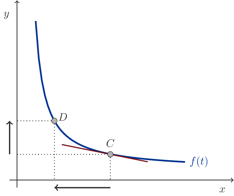
When we move on the isoquant from point \(C\) to point \(D\), we substitute a certain amount of factor \(A\) with factor \(B\) while keeping the output unchanged. From comparing the lengths of the horizontal and the vertical arrow, we can see that an increase in factor \(B\) (vertical arrow), i.e., additional machine time, means a significantly more substantial reduction in the use of factor \(A\) (horizontal arrow). Additional machine time results in a more-than-proportional saving of raw material while maintaining the same output.
We are interested in the marginal change of the factor inputs. It is nothing other than the slope \(f'(t)\) of the tangent to a point on the isoquant. Its absolute value is called the marginal rate of substitution RTS.
Exercise 8.52 Let \(F(x,y)=2x-y+6\).
Find the explicit definition of the function \(y=f(t)\), which is implicitly defined by the equation \(F(t,f(t))=-3\).
Calculate the first and the second derivative of the function \(f(t)\).
Solution: We set \(x=t\) and \(y=f(t)\) and substitute this into \(F(x,y)\): \[ \begin{gathered} F(x,y) = F(t,f(t)) = 2t - f(t) + 6 = -3, \\[1ex] \implies f(t) = 2t + 9,\qquad f'(t) = 2,\quad f''(t) = 0. \end{gathered} \] □
Exercise 8.53 Let \(F(x,y) = 20 x^{0.3} y^{0.6}\).
Determine the explicit definition of the function \(f(t)\) that is implicitly defined by the equation \(F(t,f(t)) = 2\).
Calculate the first and second derivatives of the function \(y = f(t)\).
Solution: The equation \[ \begin{gathered} F(t,f(t)) = 20t^{0.3}f(t)^{0.6} = 2 \end{gathered} \] is solved by \[ \begin{gathered} f(t)^{0.6} = \frac{2}{20t^{0.3}} = 0.1 \cdot t^{-0.3}. \end{gathered} \] and therefore \[ \begin{gathered} f(t) = \left(0.1 \cdot t^{-0.3}\right)^{1/0.6} = 0.0215 \cdot t^{-0.5} = \frac{0.0215}{\sqrt{t}}. \end{gathered} \] The derivatives are \[ \begin{gathered} f'(t) = -\frac{0.01075}{t\sqrt{t}},\quad f''(t) = \frac{0.016125}{t^2\sqrt{t}}\,. \end{gathered} \] □
The following example shows that it can sometimes be a bit tedious to determine the explicit form of a function implicitly defined.
Exercise 8.54 The production function is given by \(F(x,y) = x^2 + 5xy + y^2\). At the moment, the manufacturer uses the factor combination \((x,y) = (3,5)\). Now the use of factor \(A\) is to be increased and the use of factor \(B\) decreased, while maintaining the current production level.
Calculate the marginal rate of substitution of factor \(A\) for factor \(B\).
Solution: The production level is \(F(3,5) = 109\). We denote the amount of factor \(A\) with \(t\) and the amount of factor \(B\) with \(f(t)\).
The marginal rate of substitution is the first derivative of the function \(f(t)\), which is implicitly defined by the equation \[ \begin{gathered} F(t,f(t)) = F(3,5) = 109 \end{gathered} \] at the point \(t = 3\).
We solve this problem here by determining the explicit form of the function \(y = f(t)\). It is \[ \begin{gathered} F(t,f(t)) = t^2 + 5tf(t) + f(t)^2 = 109, \end{gathered} \] i.e., we get the quadratic equation \[ \begin{gathered} f(t)^2 + 5tf(t) + t^2 - 109 = 0, \end{gathered} \] which we must solve for \(f(t)\). This results in \[ \begin{gathered} f(t) = \frac{-5t + \sqrt{25t^2 - 4(t^2 - 109)}}{2} = \frac{\sqrt{436 + 21t^2} - 5t}{2}. \end{gathered} \] We are only interested in positive solutions. The derivative is \[ \begin{gathered} f'(t) = \frac{1}{2} \left(\frac{21t}{\sqrt{436+21t^2}} - 5\right) \end{gathered} \] By substituting \(t = 3\) we get the marginal rate of substitution for \(t = 3\): \[ \begin{gathered} f'(3) = -1.24 \implies \text{RTS} = |f'(3)| = 1.24\,. \end{gathered} \] The answer is thus: If factor \(A\) is increased by one unit, factor B must be decreased by approximately 1.24 units to maintain the production level. □
There is also a simpler solution. We differentiate the function \[ \begin{gathered} c(t) = F(t,f(t)) \end{gathered} \] using the chain rule (Theorem 8.47). We take the following path: \[ \begin{gathered} \mathbf g(t) = \left(\begin{array}{c} t \\ f(t) \end{array}\right), \quad \mathbf g'(t) = \left(\begin{array}{c} 1 \\ f'(t) \end{array}\right). \end{gathered} \] The chain rule then yields: \[ \begin{gathered} c'(t) = F'_1(t,f(t)) \cdot 1 + F'_2(t,f(t)) f'(t)\;. \end{gathered} \] Since the implicitly defined function \(f(t)\) is defined such that \(c(t)\) is constant (in the example the production level \(109\)), \(c'(t)\) must be identically zero. This leads to the formula \[ \begin{gathered} f'(t) = -\frac{F'_1(t,f(t))}{F'_2(t,f(t))}\,. \end{gathered} \] To calculate the derivative of an implicit function \(f(t)\), it is thus not necessary to compute the function \(f(t)\) explicitly. We only need the partial derivatives of the function \(F(x,y)\).
Theorem 8.55 (Derivative of Implicit Functions) Let \(F(x,y)\) and \(f(t)\) be functions with continuous derivatives. If \(c(t) = F(t,f(t)) \equiv \text{const}\), then \[ \begin{gathered} f'(t) = -\frac{F'_1(t,f(t))}{F'_2(t,f(t))}, \end{gathered} \] provided the denominator is not zero.
Let’s look at the solution to Exercise 8.54 again. We have \[ \begin{gathered} F'_1(x,y) = 2x + 5y, \quad F'_2(x,y) = 5x + 2y. \end{gathered} \] From this, for \(x = t = 3\) and \(y = f(t) = 5\), we get: \[ \begin{gathered} f'(3) = -\frac{F'_1(3,5)}{F'_2(3,5)} = -\frac{31}{25} = -1.24. \end{gathered} \] □
Exercise 8.56 The production function is given by \(F(x,y) = 100x^{0.1}y^{0.7}\). At the moment, the manufacturer uses the factor combination \((x,y) = (2,1)\). Now the use of factor \(A\) is to be increased and the use of factor \(B\) decreased, while maintaining the production level. The marginal rate of substitution of factor \(A\) for factor \(B\) is to be calculated.
Solution: We calculate the partial derivatives of the function \(F\): \[ \begin{gathered} F_1'(x,y)=10x^{-0.9}y^{0.7},\qquad F_2'(x,y)=70x^{0.1}y^{-0.3},\\[1ex] F_1'(2,1)=10\cdot 2^{-0.9},\qquad F_2'(2,1)=70\cdot 2^{0.1}. \end{gathered} \] Using the rule for derivative of implicit functions, we obtain: \[ \begin{aligned} f'(2)&=-\frac{F_1'(2,1)}{F_2'(2,1)}=-\frac{10\cdot 2^{-0.9}}{70\cdot 2^{0.1}}=-\frac{10}{70\cdot 2}=-0.0714\\ &\implies \text{RTS} =0.0714\,. \end{aligned} \] □
8.8 Optimization with Constraints
8.8.1 Introduction to the Task
In Example 8.51 we already pointed out an important aspect: Production factors have prices, therefore it is reasonable to ask how a certain output can be produced at minimal costs.
We will now examine this question.
A manufacturer produces a good using two factors (e.g., raw materials) \(A\) and \(B\). The combination of input quantities \(x,\;y\) is variable. The manufacturer’s production function is \[ \begin{gathered} q=F(x,y). \end{gathered} \] The combination of factors should now be chosen optimally, i.e., the production costs should be minimized for a given level of output.
The factor prices are \(a\) and \(b\) per unit of quantity. Therefore, the costs (excluding fixed costs) of the factor combination \((x,y)\) and thus of the output \(q=F(x,y)\) are: \[ \begin{gathered} C(x,y)=ax+by. \end{gathered} \] This linear cost function should be minimized under the constraint that the output should be exactly \(q=F(x,y)\) units.
One can solve this task by determining the implicit function \(f(t)\) defined by the production level \[ \begin{gathered} F(t,f(t))=q \end{gathered} \] Then calculate the costs of all these factor combinations \[ \begin{gathered} c(t)=at+bf(t), \end{gathered} \] and determine a critical point through the equation \[ \begin{gathered} c'(t)=a+bf'(t)=0\;. \end{gathered} \]
Exercise 8.58 The production function is \(q=F(x,y)=100\,xy\) and factor prices are 2 and 3 units of currency per unit of quantity, respectively. Determine the optimal factor combination for a production level \(q=200\).
Solution: The function \(f(t)\) is implicitly defined by \(F(t,f(t))=200\), so \[ \begin{gathered} 100tf(t)=200 \;\implies\; f(t)=\frac{2}{t}\,. \end{gathered} \] Therefore, the costs are \[ \begin{gathered} c(t)=2t+3\cdot \frac{2}{t}=2t+\frac{6}{t}, \end{gathered} \] with \(c'(t)=2-6/t^2\). We calculate the minimum by \[ \begin{gathered} c'(t)=2-\frac{6}{t^2}=0\implies t=\pm\sqrt{3}. \end{gathered} \] We therefore have a minimum at \(t=\sqrt{3}\). The optimal factor combination is thus \(x=t=\sqrt{3}\simeq 1.73\) and \(y=f(t)=2/\sqrt{3}\simeq 1.15\). □
Remark 8.59 It was not really difficult for us to find the solution in Exercise 8.58. However, we should not delude ourselves. It was only easy
Because we were able to calculate \(f(t)\) explicitly.
Thus, we reduced the objective function \(c(x,y)=2x+3y\) to a function \(c(t)\) in just one variable.
We have incorporated the constraint into the objective function.
If that is too difficult or even impossible, we have an elegant alternative, the Method of Lagrange.
8.8.2 The Method of Lagrange
Let \(z=C(x,y)\) be an objective function, which is to be optimized under the constraint \(F(x,y)=q=\text{const}\). Theoretically, we would define a function \(y=f(t)\) implicitly by the equation \[ \begin{gathered} q=F(t,f(t)) \end{gathered} \] and then look for a critical point of the objective function \[ \begin{gathered} c(t)=C(t,f(t)) \end{gathered} \] This approach can be impractical due to the complexity of the explicit form of \(f(t)\). Nevertheless, we can examine what conditions a critical point would need to satisfy.
A critical point of \(c(t)\) must satisfy the equation \(c'(t)=0\), which due to the chain rule (Theorem 8.47) is \[ \begin{gathered} C'_1(t,f(t))\cdot 1+C'_2(t,f(t))\,f'(t)=0\qquad \mbox{(A)} \end{gathered} \] On the other hand, \(f'(t)\) is the derivative of an implicitly defined function and thus, due to Theorem 8.55, it holds that \[ \begin{gathered} F'_1(t,f(t))\cdot 1+F'_2(t,f(t))\,f'(t)=0.\qquad \mbox{(B)} \end{gathered} \] Since \(f'(t)\) satisfies two linear equations (A) and (B) (linear in the unknown \(f'(t)\)) simultaneously, the coefficients of these equations must be proportional, i.e., there exists a number \(\lambda\) such that \[ \begin{aligned} C'_1(t,f(t))&=\lambda F'_1(t,f(t))\\ C'_2(t,f(t))&=\lambda F'_2(t,f(t)). \end{aligned} \]
Theorem 8.60 Let \(z=C(x,y)\) be an objective function that is to be optimized under the constraint \(F(x,y)=q\).
A point \((x,y)\) is exactly a critical point of this optimization problem if there is a number \(\lambda\) such that \[ \begin{aligned} C'_1(x,y)&=\lambda F'_1(x,y), \end{aligned} \tag{8.5}\]
\[ \begin{aligned} C'_2(x,y)&=\lambda F'_2(x,y). \end{aligned} \tag{8.6}\] The number \(\lambda\) is called Lagrange multiplier.
This condition for critical points of an optimization problem with a constraint avoids the explicit representation of the underlying implicit function \(f(t)\).
Essentially, one could stop at this rule for finding critical points and simply apply it. However, it has become customary to use a calculation scheme known as the Method of Lagrange Multipliers.
In this calculation scheme, one proceeds as follows:
Step 1: Define a new objective function \[ \begin{gathered} L(x,y,\lambda)=C(x,y)-\lambda(F(x,y)-q). \end{gathered} \] This is the so-called Lagrange function.
Step 2: Search for critical points of the Lagrange function.
A critical point of the Lagrange function is characterized by all (three!) partial derivatives of the Lagrange function (with respect to \(x\), \(y\), and \(\lambda\)) being equal to zero: \[ \begin{aligned} L'_1&=C'_1-\lambda F'_1=0\\ L'_2&=C'_2-\lambda F'_2=0\\ L'_3&=-(F-q)=0\Leftrightarrow F-q=0. \end{aligned} \] The first two equations are exactly the conditions that a critical point must satisfy according to Theorem 8.60. The third equation is simply the constraint under which optimization is to occur.
Let’s look again at the solution of Exercise 8.58.
The Lagrange function is \[ \begin{gathered} L(x,y,\lambda)=2x+3y-\lambda(100xy-200). \end{gathered} \] We form the partial derivatives with respect to \(x\) and \(y\) and set them to zero: \[ \begin{aligned} L'_1&=2-100\lambda y=0\\ L'_2&=3-100\lambda x=0 \end{aligned} \] The third equation we need is the constraint: \[ \begin{gathered} 100xy=200 \implies xy=2. \end{gathered} \] We solve the first two equations for \(x\) and \(y\) and express these solutions as functions of \(\lambda\): \[ \begin{gathered} x=\frac{0.03}{\lambda},\quad y=\frac{0.02}{\lambda}.\qquad \mbox{(A)} \end{gathered} \] We now substitute \(x\) and \(y\) into the constraint, i.e., into \(xy=2\): \[ \begin{gathered} \frac{0.0006}{\lambda^2}=2\implies \lambda=\pm\frac{\sqrt{3}}{100}. \end{gathered} \] The Lagrange multiplier can thus take on two values, which means we have two critical points after substituting into (A): \[ \begin{gathered} \lambda_1=\frac{\sqrt{3}}{100},\quad x_1=\sqrt{3},\quad y_1=\frac{2}{\sqrt{3}}, \end{gathered} \] and \[ \begin{gathered} \lambda_2=-\frac{\sqrt{3}}{100},\quad x_2=-\sqrt{3},\quad y_2=-\frac{2}{\sqrt{3}}, \end{gathered} \] Now we face a problem: we have not formulated any second-order conditions for the Lagrange problem, comparable to Theorem 8.36 and Theorem 8.41. These conditions allowed us to classify critical points as maxima or minima.
Indeed, it is possible to specify such conditions for the current case as well. However, these conditions are simply too complicated for us, so we have to find some other way out.
The simplest way seems to be to calculate the value of the objective function \(C(x,y)\) for both critical points and choose the point that delivers the better value of the objective function. Better means, for a maximum the higher, for a minimum the lower value.
In our example, \(C(x,y)=2x+3y\): \[ \begin{gathered} C\left(\sqrt{3},\frac{2}{\sqrt{3}}\right)=2\sqrt{3}+\frac{6}{\sqrt{3}}= 4\sqrt{3}=6.92820\\ C\left(-\sqrt{3},-\frac{2}{\sqrt{3}}\right)=-2\sqrt{3}-\frac{6}{\sqrt{3}}= -4\sqrt{3}=-6.92820 \end{gathered} \] However, we immediately realize that this approach is not promising in our example. Because according to this rule, we would have to take the critical point corresponding to \(\lambda_2=-\sqrt{3}/100\), but the associated values of \(x\) and \(y\) are both negative, thus economically implausible, because \(x\) and \(y\) are quantities which must be nonnegative.
In our situation, it is therefore better to argue with economic plausibility: due to the nonnegativity requirement we choose the solution corresponding to \(\lambda_1\), i.e. \(x=\sqrt{3}\simeq 1.73,y=2/\sqrt{3}\simeq 1.15\).
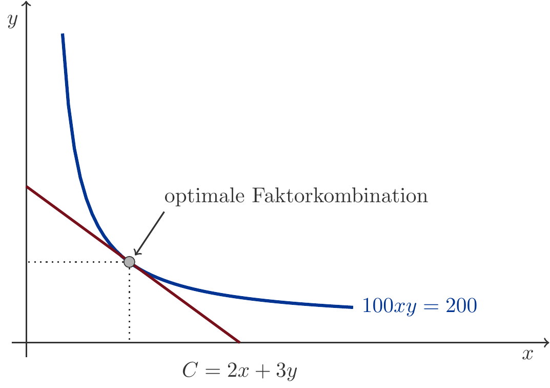
In Figure 8.13, the solution is graphically depicted. The isoquant of the production function at level \(q=200\) and an isocost line of the cost function \(C(x,y)=2x+3y\) are drawn in, precisely the one that touches the isoquant of the production function. This point of contact is the optimum.
8.8.3 Economic Interpretation of the Lagrange Multiplier
Let’s take another look at the Lagrange function: \[ \begin{gathered} L(x,y,\lambda)=C(x,y)-\lambda(F(x,y)-q), \end{gathered} \] but this time our interest is in the magnitude \(q\) in the constraint. In economic applications, \(q\) often represents a capacity constraint, i.e., a resource is not available indefinitely but in a constrained amount \(q\). In the last example (Exercise 8.58), \(q=200\) could be the maximum amount that can be produced given the existing technical equipment.
If we now change the value of \(q\), then the location of the optimum will change as well. In other words: both \(x\) and \(y\) are functions of \(q\)! Assume we have found an optimum with the values \(\lambda\), \(x^\ast\) and \(y^\ast\). Then these values depend functionally on \(q\) and we should write: \[ \begin{gathered} \lambda=\lambda(q),\quad x^\ast=x^\ast(q),\quad y^\ast=y^\ast(q). \end{gathered} \] But this also means that the value of the objective function \(C(x,y)\) at the optimum depends on \(q\): \[ \begin{gathered} C(x^\ast,y^\ast)=C^\ast(q). \end{gathered} \] Now something very remarkable can be shown3: the Lagrange multiplier is nothing other than the rate of change of \(C^\ast(q)\) with respect to \(q\): \[ \begin{gathered} \frac{d C^\ast(q)}{dq}=\lambda(q), \end{gathered} \tag{8.7}\] \(\lambda(q)\) is thus the first derivative of \(C^\ast(q)\) with respect to \(q\) and tells us at what rate the objective function \(C^\ast(q)\) increases or decreases when we loosen or tighten the capacity constraint \(q\). If we change \(q\) by a small amount \(h\), then approximately due to the principle of local linearization (see 3.9): \[ \begin{gathered} C^\ast(q+h)-C^\ast(q)\approx \lambda(q)h.\qquad \mbox{(A)} \end{gathered} \] Indeed, the multiplier \(\lambda(q)\) has the character of a price, it is also referred to as the shadow price of a constrained resource.
Let’s return one last time to Exercise 8.58. Here \(q=200\) was given and we found \[ \begin{gathered} \lambda(200)=\sqrt{3}/100=0.01732,\quad\text{with } C^\ast(200)=4\sqrt{3}=6.92820\,. \end{gathered} \] An increase in \(q\) will therefore (because \(\lambda>0\)) also lead to an increase in the cost minimum, but this will be quite small, because \(\lambda\) has a low value. To see this, let us repeat the calculation with \(q=201\), thus increasing the output level by one unit, i.e., \(h=1\) in (A). Then our computation gives: \[ \begin{gathered} \lambda(201)=0.01728, \quad\text{with } C^\ast(201)=6.94550\,. \end{gathered} \] And indeed, \[ \begin{gathered} C^\ast(201)-C^\ast(200)=0.0173\simeq \lambda(200). \end{gathered} \]
We conclude this chapter with another example.
Exercise 8.61 The production function of a manufacturer is given by \(F(x,y)=x^2+5xy+y^2\). Determine the optimal factor combination for the factor prices 15 and 20 and the production level 2500.
Solution: The Lagrange function is \[ \begin{gathered} L(x, y, \lambda) = 15x + 20y - \lambda(x^2 + 5xy + y^2 - 2500). \end{gathered} \] We form the partial derivatives and set them equal to zero: \[ \begin{aligned} L'_1 &= 15 - \lambda(2x + 5y) = 0\\ L'_2 &= 20 - \lambda(5x + 2y) = 0 \end{aligned} \] As the third equation we have the constraint: \[ \begin{gathered} x^2 + 5xy + y^2 = 2500. \end{gathered} \] The first two equations form a linear system of equations \[ \begin{gathered} 2x + 5y = \frac{15}{\lambda},\quad 5x + 2y = \frac{20}{\lambda}. \end{gathered} \] We solve this system of equations and express the solutions \(x\) and \(y\) as functions of \(\lambda\): \[ \begin{gathered} x = \frac{10}{3\lambda},\quad y = \frac{5}{3\lambda}.\qquad \mbox{(A)} \end{gathered} \] We substitute this into the constraint: \[ \begin{gathered} \frac{100}{9\lambda^2} + \frac{250}{9\lambda^2} + \frac{25}{9\lambda^2} = 2500 \implies \lambda^2 = \frac{375}{22500} \implies \lambda = \pm 0.1291. \end{gathered} \] Again, the Lagrange multiplier has two possible values, but only the positive value \(\lambda = 0.1291\) is of interest, because it guarantees positive solutions4. Substituting into (A) we obtain the cost minimum at: \[ \begin{gathered} x = \frac{10}{3 \cdot 0.1291} = 25.82,\quad y = \frac{5}{3 \cdot 0.1291} = 12.91 \end{gathered} \] See Figure 8.14 for an illustration.
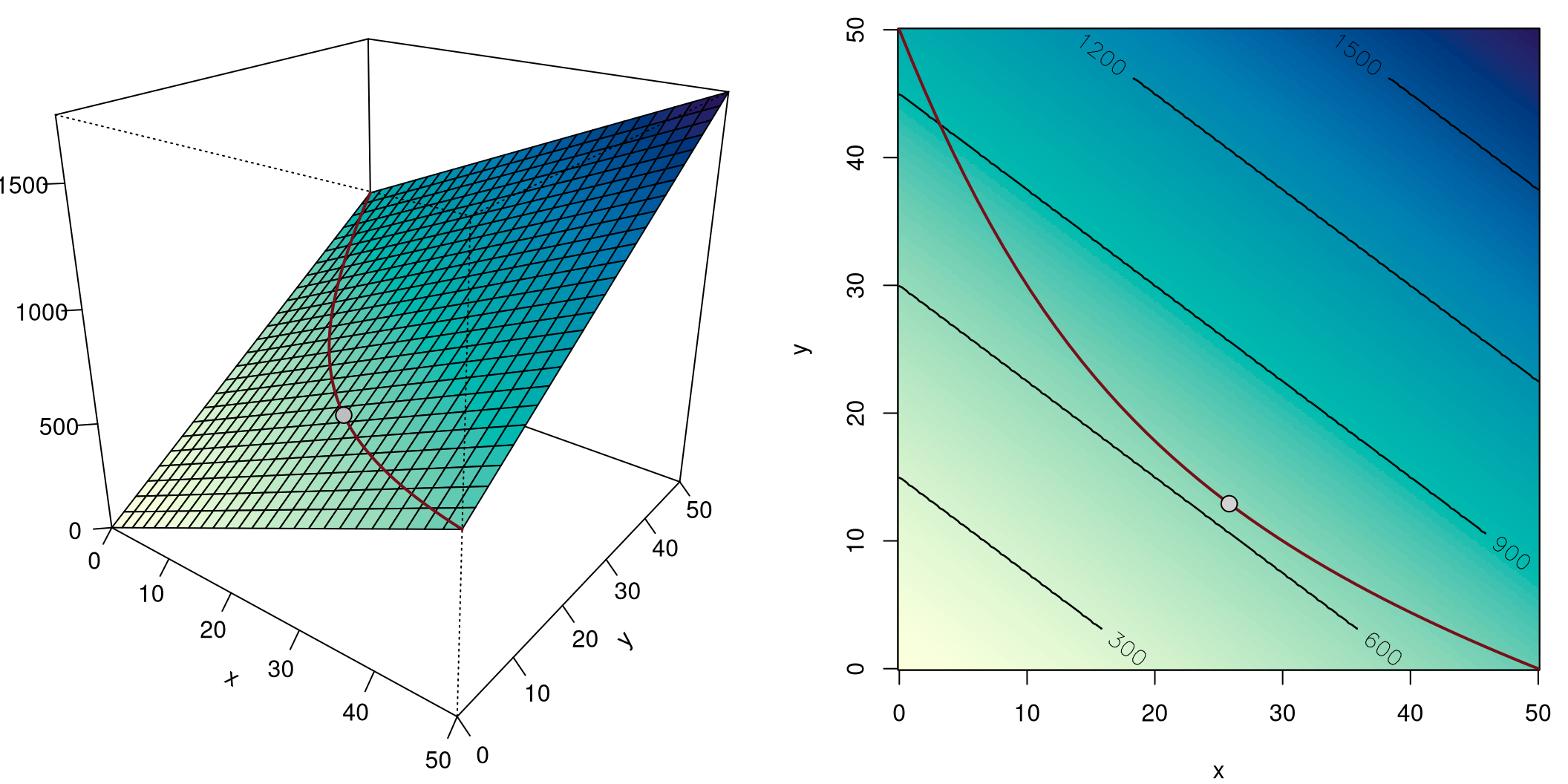
8.9 Additional Exercises
-
Determine the first partial derivatives of \(f(x, y) = \sqrt{x/y}\) at the point \({\mathbf a}^\top = (2, 5)\).
Solution: \(\displaystyle f_1'(x, y) = \frac{1}{2\sqrt{xy}}, \;f_2'(x, y) = -\frac{\sqrt{x}}{2y\sqrt{y}}\),
\(f_1'(2, 5) = 0.1581,\;f_2'(2, 5) = -0.0623\) -
Determine the first partial derivatives of \(f(x, y) = e^{x^2 + xy + y^2}\) at the point \({\mathbf a}^\top = (0, 1)\).
Solution: \(\displaystyle f_1'(x, y) = (2x + y)e^{x^2 + xy + y^2},\;f_2'(x, y) = (x + 2y)e^{x² + xy + y²}\),
\(f_1'(0, 1) = 2.7183,\;f_2'(0, 1) = 5.4366\) -
Determine the first partial derivatives of \(f(x, y) = x^y\) at the point \({\mathbf a}^\top = (1, 0)\).
Solution: \(f_1'(x, y) = y\,x^{y - 1},\;f_2'(x, y) = x^y \ln x\),
\(f_1'(1, 0) = 0,\;f_2'(1, 0) = 0\). -
Determine the first partial derivatives of \(f(x, y) = x^2 \ln(xy)\) at the point \({\mathbf a}^\top = (2, 2)\).
Solution: \(\displaystyle f_1'(x, y) = 2x \ln(xy) + x,\;f_2'(x, y) = \frac{x^2}{y}\),
\(f_1'(2, 2) = 7.5452,\;f_2'(2, 2) = 2\) -
Determine the directional derivative of \(f(x,y)=e^{x-y}\) along the uniform motion \(\mathbf x=\mathbf a+t\mathbf v\) with \({\mathbf a}^\top =(0,0)\) and \({\mathbf v}^\top =(1,1)\) at \(t=0\).
Solution: \(0\)
-
Determine the directional derivative of \(f(x,y)=x^2-5y\) along the uniform motion \(\mathbf x=\mathbf a+t\mathbf v\) with \({\mathbf a}^\top =(1,0)\) and \({\mathbf v}^\top =(-1,2)\) at \(t=0\).
Solution: \(-12\)
-
What is the value of the Hessian matrix of the function \(f(x,y)=e^{x^2+2y}\) at the point \((0,0)\)?
Solution: \(\displaystyle \boldsymbol{f}''(x,y)=e^{x^2+2y}\left(\begin{array}{cc}2+4x^2 & 4x\\4x & 4\end{array}\right),\; \boldsymbol{f}''(0,0)=\left( \begin{array}{cc}2 & 0\\0 & 4\end{array}\right)\).
-
What is the value of the Hessian matrix of the function \(f(x,y)=\sqrt{xy}\) at the point \((1,1)\)?
Solution: \(\displaystyle \boldsymbol{f}''(x,y)=\left(\begin{array}{cc}-\frac{\sqrt{y}}{4x\sqrt{x}} & \frac{1}{4\sqrt{xy}}\\\frac{1}{4\sqrt{xy}} & -\frac{\sqrt{x}}{4y\sqrt{y}} \end{array}\right)\),
\(\displaystyle \boldsymbol{f}''(1,1)=\frac{1}{4}\left( \begin{array}{rr}-1 & 1\\1 & -1\end{array}\right)\). -
What is the value of the Hessian matrix of the function \[ \begin{gathered} f(x,y)=-2x^{2} y^{3}+5x^{2} y^{2}+5x y^{2}+4x y+2 \end{gathered} \] at the point \((-1,1)\)?
Solution: \(\displaystyle\boldsymbol{f}''(1,1)=6\left( \begin{array}{rr}1 & 1\\1 & -2\end{array}\right)\).
-
Let \(\displaystyle q(p_1,p_2)=\frac{10}{p_1p_2}\) be the demand function for a good \(Q\) depending on its price \(p_1\) and the price \(p_2\) of a competing product. Calculate the partial price elasticities w.r.t. \(p_1\) and \(p_2\).
Solution: \(\epsilon_1(p_1,p_2)=\epsilon_2(p_1,p_2)=-1\)
-
Find the global extreme values of the function \[ \begin{gathered} f(x,y) = 7x^{2} +10x y-102x +9 y^{2}-138 y+9. \end{gathered} \]
Solution: Minimum at \((3,6)\).
-
Find the global extreme values of the function \[ \begin{gathered} f(x,y) = -10x^{2} -6x y-32x -6 y^{2}+72 y+8. \end{gathered} \]
Solution: Maximum at \((-4,8)\).
-
A monopoly company offers two goods at prices \(p_1\) and \(p_2\). The demand is determined by the demand functions \[ \begin{aligned} q_1&=D_1(p_1,p_2)=400-2p_1+p_2\\ q_2&=D_2(p_1,p_2)=280+p_1-5p_2 \end{aligned} \] The production costs (excluding fixed costs) of the goods are 14 and 20 CU, respectively. What prices will maximize the profit?
Solution: \(p_1=401/3,\,p_2=190/3\).
-
A monopoly company offers two goods at prices \(p_1\) and \(p_2\). The demand is determined by the demand functions \[ \begin{aligned} q_1&=D_1(p_1,p_2)=850-p_1-p_2\\ q_2&=D_2(p_1,p_2)=780-p_1-3p_2 \end{aligned} \] The production costs (excluding fixed costs) of the goods are 28 and 44 CU, respectively. What prices will maximize the profit?
Solution: \(p_1=456.5,\,p_2=4.5\).
-
Let \(f(x,y)=3x e^{-2y}\) and \(\mathbf x=\mathbf g(t)\) with \(g_1(t)=-8 t^2\) and \(g_2(t)=2\ln t\). Determine \(c'(1.2)\) for \(c(t)=f(\mathbf g(t))\).
Solution: \(c'(1.2)=27.78\)
-
The production function of a company is \[ \begin{gathered} F(x,y)=3x^{2} +2x y+3 y^{2}, \end{gathered} \] where \(x\) and \(y\) represent the quantities used of the two production factors \(A\) and \(B\) respectively. Currently, the manufacturer is using the factor combination \((x,y)= (7,5)\). They now wish to increase the use of factor \(A\) and decrease the use of factor \(B\), while maintaining the production level. Calculate the marginal rate of substitution of factor \(A\) for factor \(B\).
Solution: \(1.18\)
-
Find the maximum of the function \(F(x,y)=xy\) subject to the constraint \(5x+2y=20\).
Solution: \(x=2, y=5\).
-
Find the minimum of the function \(F(x,y)=x^2+y^2\) subject to the constraint \(2x+3y=26\).
Solution: \(x=4, y=6\).
-
The production function of a company is \[ \begin{gathered} F(x,y)=2x^{2} +14x y+4 y^{2}, \end{gathered} \] where \(x\) and \(y\) represent the amounts of the two production factors \(A\) and \(B\) respectively. The prices of production factors are 15 and 19 CU per unit quantity, respectively. Calculate the quantities of production factors used when 6400 units of the final product are manufactured at minimum costs.
Solution: \(x=18.74,\,y=17.20\).
-
The production function of a company is given by \[ \begin{gathered} F(x,y)=173 x^{0.65} y^{0.43}, \end{gathered} \] where \(x\) and \(y\) are the quantities of the two production factors \(A\) and \(B\) respectively. The prices of the production factors are 20 and 10 MU per unit respectively. Calculate the quantities of production factors used if 9500 units of the final product are to be manufactured at minimal cost.
Solution: \(x=36.51,\,y=48.30\).