4 Integration
4.1 Antiderivatives and Integrals
4.1.1 Preliminaries
The main concern of differential calculus is to make precise statements about the changing behavior of a function. However, ever since the discovery of differential calculus in the 17th century, this problem was seen in conjunction with the question: How can one reconstruct a function from its known changing behavior?
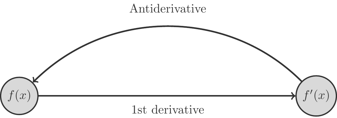
This question leads us to a first interpretation of the concept of integral: if we know the first derivative \(f'(x)\) of a function \(f(x)\), how can we determine \(f(x)\)? So, initially, it is about reversing the process of differentiation. Therefore, \(f(x)\) is also called the antiderivative or better the antifunction of \(f'(x)\). We can illustrate the situation schematically like this:

Now, as we have seen, the process of differentiation is a very simple one; it is just a handful of rules that we can apply in almost a mechanical way. Therefore, we expect that the reversal of this process, the finding of the antiderivative, is just as simple. But unfortunately, it is a bit more complicated. However, in this chapter, we will learn methods that, with some practice and skill, in many cases (although not in all) will provide us with the antiderivative of a given function.
In this chapter, we will give a second meaning to the concept of integral, namely as a solution to a quadrature problem. This refers to the calculation of the area between the graph of a function \(f(x)\) and the x-axis. It is also referred to as the determined integral. This naturally raises the question: how do these two interpretations of the integral concept, the antiderivative and the solution to a quadrature problem, relate?
This connection is established by the Fundamental Theorem of Calculus, a crown jewel of mathematics that we owe to Isaac Newton and Gottfried Leibniz.
4.1.2 Antiderivatives
Definition 4.1 Let \(F(x)\) be a differentiable function and let \(f(x)=F'(x)\) be its derivative. Then \(F(x)\) is called an antiderivative of \(f(x)\).
Clearly, \(F(x)=x^2\) is an antiderivative of \(f(x)=2x\). But also \(G(x)=x^2+3\) is an antiderivative of \(f(x)=2x\).
Antiderivatives are obviously not uniquely determined. For every function \(f(x)\) that has an antiderivative \(F(x)\), there are infinitely many other antiderivatives. But these antiderivatives do not differ very much.
Theorem 4.3 If \(F(x)\) and \(G(x)\) are two antiderivatives of the same function \(f(x)\), then \(F\) and \(G\) differ only by an additive constant, that is \(F(x)=G(x)+C\).
Justification: From \(F'(x)=G'(x)\) it follows that \(F'(x)-G'(x)=0\). Now, on the left side of this equation is the derivative of the difference \(F(x)-G(x)\), and on the right side is zero, thus the derivative of a constant. Hence, \(F(x)-G(x)\) must be constant. □
4.1.3 Determined Integrals
Antiderivatives are closely related to determined integrals. We explain the concept of the determined integral using an example from financial mathematics.
Let \(K(t)\) be the amount of capital, which changes in the time interval \([0,T]\). We denote the derivative, that is, the rate of change of the capital \(K(t)\) by \(k(t)=K'(t)\). The amount of capital is thus an antiderivative of the rate of change of the capital.
In Section 3.3.3, we discussed the fundamental concept of local linearization of functions. This proves once again to be very helpful. Assume \([t_1,t_2]\) is an interval. Then approximately the following relationship holds \[ \begin{gathered} K(t_2)\approx K(t_1)+k(t_1)(t_2-t_1). \end{gathered} \] This equation can be interpreted as follows: On a very small time interval \([t_1,t_2]\), the rate of change can be considered approximately constant at \(k(t_1)\). If such a constant rate of change \(k(t_1)\) acts over the time interval \([t_1,t_2]\), then the capital changes by \(k(t_1)(t_2-t_1)\).
How can one now reconstruct the course of the capital \(K(t)\) from the given rate of change \(k(t)\) in reverse? This process is called integrating.
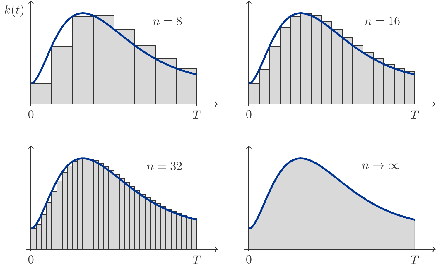
To better understand the process of integration, let’s imagine that the time interval \([0,T]\) is divided into subintervals \[ \begin{gathered} 0=t_0<t_1<t_2<\ldots<t_{n-1}<t_n=T. \end{gathered} \] Then it is clear that \[ \begin{aligned} K(T)-K(0)=\;&[K(t_1)-K(t_0)]+[K(t_2)-K(t_1)] +\cdots+ \\ &[K(t_n)-K(t_{n-1})]. \end{aligned} \] For each of the individual small subintervals \([t_{i-1},t_i]\), we assume that the rate of change starting with the left endpoint is approximately constant at \(k(t_{i-1})\). Then, according to our approximation formula, we obtain \[ \begin{gathered} K(t_i)\approx K(t_{i-1})+k(t_{i-1})(t_i-t_{i-1}), \end{gathered} \] and therefore \[ \begin{gathered} \begin{array}{rcl} K(T)-K(0) & \approx & k(t_0)(t_1-t_0)+k(t_1)(t_2-t_1) \\ & & +\cdots+ k(t_{n-1})(t_n-t_{n-1})\\[2pt] & = & \displaystyle \sum_{i=1}^n k(t_{i-1})(t_i-t_{i-1}). \end{array} \end{gathered} \tag{4.1}\] This is, of course, only an approximation formula. The meaning of (4.1) is graphically represented in Figure 4.2. It shows that (4.1) corresponds to the area of the gray rectangular strips and becomes more accurate with increasing \(n\). In order to convert (4.1) into an exact equation, we need to let the length of the subintervals converge to zero, which simultaneously means that the number of subintervals tends towards infinity.
Under certain conditions, it is indeed the case that the sum on the right side converges to a limit. This limit is denoted by the symbol
\[ \begin{gathered} \int_0^T k(t)\,\mathrm{d}t \end{gathered} \]
(This is a stylization of the summation notation) and is called an integral. This limit corresponds to the area underneath the graph of the function \(k(t)\) and thus solves a quadrature problem.
With this notation, we obtain the formula
\[ \begin{gathered} K(T)=K(0)+\int_0^T k(t)\,\,\mathrm{d}t. \end{gathered} \tag{4.2}\] This equation is read as follows: The final capital \(K(T)\) is obtained from the initial capital by integrating the rate of change \(k(t)\), that is, by summing up the rate of change \(k(t)\), weighted with the lengths \(\mathrm{d}t\) of the subintervals on which the rate of change \(k(t)\) is effective.
But how are antiderivatives and integrals related?
Theorem 4.5 (Fundamental Theorem of Calculus) Let \(f(x)\) be a function that has an antiderivative \(F(x)\) and let \(a,b\in\mathbb R\). Then the following holds \[ \begin{gathered} \int_a^b f(x)\,\,\mathrm{d}x := F(b)-F(a) = F(x)\Big|_a^b, \end{gathered} \tag{4.3}\] and equation (4.3) is called the definite integral of \(f\) between the limits \(a\) and \(b\).
A consequence of (4.1) is the additivity of the integral:
Theorem 4.6 (Additivity) If \(a<b<c\), then the following holds: \[ \begin{gathered} \int_a^c f(x)\,\mathrm{d}x=\int_a^b f(x)\,\mathrm{d}x+\int_b^c f(x)\,\mathrm{d}x. \end{gathered} \]
It does not matter which specific antiderivative of \(f(x)\) you use for the definition or calculation of an integral. Since different antiderivatives can only differ by an additive constant, the difference \(F(b)-F(a)\) has the same value for all antiderivatives \(F(x)\) of a function \(f(x)\).
It is also important to realize that it is completely irrelevant which letter is used to represent the variable of integration. Therefore, the following terms are all equivalent: \[ \begin{gathered} \int_a^b f(x)\,\,\mathrm{d}x=\int_a^b f(y)\,\,\mathrm{d}y=\int_a^b f(t)\,\,\mathrm{d}t= \int_a^b f(u)\,\,\mathrm{d}u\,. \end{gathered} \] Obviously, it is also true that \[ \begin{gathered} \int_a^b f(x)\,\,\mathrm{d}x =-\int_b^a f(x)\,\,\mathrm{d}x, \end{gathered} \] meaning: If one exchanges the limits of integration, the sign of the integral changes.
Drawing from the symbol for the definite integral, one uses the notation \[ \begin{gathered} \int f(x)\,\,\mathrm{d}x:=F(x)+C \end{gathered} \] to denote an arbitrary antiderivative \(F\) of \(f\) and calls the expression an indefinite integral. The number \(C\) is called the constant of integration.
4.2 Methods of Calculation
Firstly, let us establish that it is only possible to represent antiderivatives of few functions with mostly simple terms as closed expressions. If this is not possible, antiderivatives must be represented by integrals, which in turn can only be approximately calculated by sums.
But sometimes it is possible to calculate antiderivatives as algebraic expressions. Such cases and methods will be discussed in this section.
Before we go into details, let’s formulate a very general rule that is an immediate consequence of Definition 4.1:
Every differentiation formula is at the same time a formula for an antiderivative. We just have to read this formula from right to left.
4.2.1 Basic Rules for Integration
We start with the differentiation formula for general powers (Theorem 3.34):
Theorem 4.7 (Powers) If \(\alpha\neq -1\), then \[ \begin{gathered} (x^{\alpha+1})'=(\alpha+1)x^\alpha \quad\implies\quad \int x^\alpha\,dx =\frac{x^{\alpha+1}}{\alpha+1}+C. \end{gathered} \tag{4.4}\]
With this formula, we can determine an antiderivative for all arbitrary powers, as long as the exponent \(\alpha\neq 1\) is not equal to 11. In particular, this formula also applies for \(\alpha=0\): \[ \begin{gathered} \int x^0\,\mathrm{d}x = \int 1\,\mathrm{d}x = x + C. \end{gathered} \tag{4.5}\]
Exercise 4.8
- Determine an antiderivative of \(f(x)=x^5\).
- Calculate \(\displaystyle\int_{-2}^3 x^5 \,\,\mathrm{d}x\).
Solution: An antiderivative is obtained by \[ \begin{gathered} F(x)=\int x^5\,\,\mathrm{d}x= \frac{x^6}{6}+C. \end{gathered} \] The definite integral is, due to the Fundamental Theorem of Calculus (Theorem 4.5): \[ \begin{gathered} \int_{-2}^3 x^5 \,\,\mathrm{d}x=F(3)-F(-2)=\frac{x^6}{6}\Big|_{-2}^3= \frac{3^6}{6}-\frac{(-2)^6}{6}=\frac{665}{6}\,. \end{gathered} \] □
Exercise 4.9
- Determine an antiderivative of \(g(u)=\frac{1}{\sqrt{u}}\).
- Calculate \(\displaystyle\int_1^{10} \frac{1}{\sqrt{u}}\,\mathrm{d}u\).
Solution: We apply (4.4) with \(\alpha=-1/2\): \[ \begin{gathered} \int \frac{1}{\sqrt{u}}\,\mathrm{d}u=\int u^{-1/2}\,\mathrm{d}u= \frac{u^{1/2}}{1/2}=2\sqrt{u}+C. \end{gathered} \] The definite integral is \[ \begin{gathered} \int_1^{10} \frac{1}{\sqrt{u}}\,\mathrm{d}u=2\sqrt{u}\Big|_1^{10}= 2\sqrt{10}-2\sqrt{1}=4.325\,. \end{gathered} \] □
The following rule shows us that finding the antiderivative, just like differentiating, is a linear operation.
Theorem 4.10 (Sum Rule) \[ \begin{gathered} \int (af(x)+bg(x))\,dx=a\int f(x)\,dx+b\int g(x)\,dx+C. \end{gathered} \] This rule has two messages for us:
- We may pull a constant factor in front of the integral.
- The integral of a sum of functions is the sum of the integrals.
Exercise 4.11
- Determine an antiderivative of \(\displaystyle f(x)=3x^2-5+\frac{1}{x^3}\).
- Calculate \(\displaystyle \int_3^7 f(x)\,\,\mathrm{d}x\).
Solution: We apply the sum rule (Theorem 4.10): \[ \begin{aligned} F(x)&=\int (3x^2-5+\frac{1}{x^{3}})\,\,\mathrm{d}x =3\int x^2\,\mathrm{d}x-5\int 1\,\mathrm{d}x+\int x^{-3}\,\mathrm{d}x\\ &=3\frac{x^3}{3}-5x+\frac{x^{-2}}{-2}+C=x^3-5x-\frac{1}{2x^2}+C. \end{aligned} \] The definite integral is valued at: \[ \begin{gathered} \int_3^7 f(x)\,\mathrm{d}x=\left[x^3-5x-\frac{1}{2x^2}\right]\Bigg|_3^7=296.045\,. \end{gathered} \]
We remember: every differentiation formula is also a formula for an antiderivative. With this, we can immediately specify antiderivatives for the Eulerian exponential function and the natural logarithm.
Theorem 4.12 (Exponential Function and Logarithm) For exponential function and logarithm apply: \[ \begin{gathered} (e^x)'=e^x \quad\implies\quad \int e^x\,\mathrm{d}x=e^x+C, \end{gathered} \] and \[ \begin{gathered} (\ln(x))'=\frac{1}{x}\quad\implies\quad \int \frac{1}{x}\,\mathrm{d}x=\ln(x)+C,\quad x>0. \end{gathered} \]
However, these rules alone are not yet very useful. We additionally need those integration rules that arise from the product rule and the chain rule for differentiation.
4.2.2 Partial Integration
Let \(f(x)\) be a function expression that does not directly yield an antiderivative. We now assume that this function term is the product of two factors \[ \begin{gathered} f(x)=g(x)h(x), \end{gathered} \] that have the following properties:
For the factor \(g(x)\), an antiderivative \(G(x)\) can be directly specified.
The factor \(h(x)\) has the derivative \(h'(x)\).
If we apply the product rule to \(G(x)h(x)\): \[ \begin{gathered} (G(x)h(x))'=g(x)h(x)+G(x)h'(x), \end{gathered} \] and go to antiderivatives, we then obtain another important rule:
Theorem 4.13 (Partial Integration) \[ \begin{gathered} \int g(x)h(x)\,\mathrm{d}x=G(x)h(x)-\int G(x)h'(x)\,\mathrm{d}x. \end{gathered} \tag{4.6}\]
We have thereby shifted the original problem: Instead of integrating \(f(x)=g(x)h(x)\), we must now integrate the function \(G(x)h'(x)\). If we have chosen the factors wisely, then it is possible that the new problem is simpler than the old one.
Exercise 4.14
- Determine an antiderivative of \(f(x)=x\ln x\).
- Calculate the integral \(\displaystyle\int_{1}^2 x\ln x\,\mathrm{d}x\).
Solution: The function \(f(x)\) is a product of the factors \(x\) and \(\ln(x)\). Since we can only directly specify an antiderivative for \(x\) (namely \(x^2/2\)), we choose in (4.6) \(g(x)=x\) and \(h(x)=\ln x\). With this choice: \[ \begin{aligned} %% {alignat*}{2} g(x)&=x &\qquad G(x)&=\frac{x^2}{2}\\[4pt] h(x)&=\ln x & h'(x)&=\frac{1}{x},\end{aligned} \] we find: \[ \begin{aligned} \int x\ln x\,\mathrm{d}x&=\frac{x^2}{2}\ln x-\int \frac{x^2}{2} \cdot\frac{1}{x}\,\mathrm{d}x\\[4pt] &=\frac{x^2}{2}\ln x-\int \frac{x}{2}\,\mathrm{d}x\\ &=\frac{x^2}{2}\ln x-\frac{x^2}{4}+C. \end{aligned} \] The definite integral amounts to \[ \begin{gathered} \int_1^2 x\ln x\,\mathrm{d}x=\frac{x^2}{2}\ln x-\frac{x^2}{4}\Bigg|_1^2=2\ln 2-\frac{3}{4}= 0.6363\,. \end{gathered} \] □
Exercise 4.15
- Determine an antiderivative of \(f(x)=xe^x\).
- Calculate the integral \(\displaystyle \int_{-1}^1 xe^x\,\mathrm{d}x\).
Solution: In this case, an antiderivative can be directly specified for both factors. It is usually appropriate to let that factor play the role of \(h(x)\), which simplifies more upon differentiating. In the present case, we therefore choose \(h(x)=x\) and \(g(x)=e^x\). With this choice: \[ \begin{aligned} g(x)&=e^x &\qquad G(x)&=e^x\\[4pt] h(x)&=x & h'(x)&=1,\end{aligned} \] we find: \[ \begin{aligned} \int xe^x\,\mathrm{d}x&=xe^x-\int e^x\,\mathrm{d}x\\ &=xe^x-e^x+C=e^x(x-1)+C. \end{aligned} \] The definite integral amounts to \[ \begin{gathered} \int_{-1}^1 xe^x\,\mathrm{d}x = e^x(x-1)\Big|_{-1}^1=2e^{-1} =0.7358\,. \\ \end{gathered} \] □
Exercise 4.16
- Determine an antiderivative of \(f(x)=\ln x\).
- Calculate the integral \(\displaystyle \int_{1}^2 \ln x\,\mathrm{d}x\).
Solution: At first glance, it is not immediately clear that this problem can be solved by partial integration. But upon closer inspection, we recognize that we can write \(\ln x=1\cdot \ln x\)! Our approach \[ \begin{aligned} g(x)&=1 &\qquad G(x)&=x\\[2pt] h(x)&=\ln x & h'(x)&=\frac{1}{x}, \end{aligned} \] yields: \[ \begin{aligned} \int \ln x\,\mathrm{d}x&=x\ln x-\int x\cdot\frac{1}{x}\,\mathrm{d}x =x\ln x-\int 1\,\mathrm{d}x\\ &=x\ln x -x+C. \end{aligned} \] With the given integration boundaries: \[ \begin{gathered} \int_1^2\ln x\,\mathrm{d}x=x\ln x-x\bigg|_1^2=2\ln 2-1=0.3863\,. \end{gathered} \] □
4.2.3 The Substitution Rule
Our experiences from Chapter 3 have shown us that the chain rule is the most important rule of differentiation. But since every rule for deriving a function provides a formula for an antiderivative, we expect that there must also be an equivalent for the chain rule.
Let \(H\) be an antiderivative of \(h\) and let \(g\) be another differentiable function. Then the chain rule states that \[ \begin{gathered} H(g(x))'=h(g(x))g'(x). \end{gathered} \] When rewritten as a statement about antiderivatives, it states \[ \begin{gathered} \int h(g(x))g'(x)\,dx= H(g(x))+C. \end{gathered} \tag{4.7}\] Suppose we are looking for \(\int h(x)\,\mathrm{d}x\), and an antiderivative \(H(x)\) is not readily available (e.g., through partial integration).
Then we can try a substitution!
We set \(x=g(t)\), and due to the chain rule, we have: \[ \begin{gathered} \int h(x)\,\mathrm{d}x=\int h(g(t))g'(t)\,\mathrm{d}t. \end{gathered} \tag{4.8}\] With a clever choice of the function \(g(t)\), the integral on the right side of (4.8) can be substantially simpler than the integral on the left side.
Let’s try this out with a classic textbook example.
Exercise 4.17
- Determine an antiderivative of \(f(x)=2xe^{x^2}\).
- Calculate \(\displaystyle\int_0^3 f(x)\,\mathrm{d}x\).
Solution: We set \(x^2 =t\) and thus get the substitution \[ \begin{gathered} x=\sqrt{t}=g(t),\qquad g'(t)=\frac{1}{2\sqrt{t}}. \end{gathered} \] We insert this: \[ \begin{aligned} \int 2xe^{x^2}\,\mathrm{d}x&=\int 2\sqrt{t}\cdot e^t\cdot \frac{1}{2\sqrt{t}} \,\mathrm{d}t. \end{aligned} \] However, the term \(2\sqrt{t}\) cancels out, so we can immediately specify an antiderivative: \[ \begin{gathered} \int 2xe^{x^2}\,\mathrm{d}x=\int 2\sqrt{t}\cdot e^t\cdot \frac{1}{2\sqrt{t}} \,\mathrm{d}t =\int e^t\,\mathrm{d}t = e^t+C \end{gathered} \] But \(t\) was just a temporary abbreviation for \(x^2\). As a final step we resubstitute \(t=x^2\) and finally find without any trouble: \[ \begin{gathered} \int 2xe^{x^2}\,\mathrm{d}x=e^{x^2}+C. \end{gathered} \] In conclusion, we insert the integration boundaries: \[ \begin{gathered} \int_0^3 f(x)\,\mathrm{d}x=e^{x^2}\Big|_0^3=e^9-1 =8102.08\,. \end{gathered} \] □
Exercise 4.18
- Determine an antiderivative of \(f(x)=\dfrac{x}{1+x^2}\).
- Calculate \(\displaystyle\int_{-2}^3 f(x)\,\mathrm{d}x\).
Solution: We set \(1+x^2 =t\) and hence get the substitution \[ \begin{gathered} x=\sqrt{t-1}=g(t),\qquad g'(t)=\frac{1}{2\sqrt{t-1}}. \end{gathered} \] This substitution results in: \[ \begin{aligned} \int \frac{x}{1+x^2}\,\mathrm{d}x&=\int \frac{\sqrt{t-1}}{t} \cdot \frac{1}{2\sqrt{t-1}}\,\mathrm{d}t=\frac{1}{2}\int \frac{1}{t}\,\mathrm{d}t =\frac{1}{2}\ln t+C. \end{aligned} \] Resubstitution \(t=1+x^2\) ultimately yields: \[ \begin{gathered} \int \frac{x}{1+x^2}\,\mathrm{d}x=\frac{1}{2}\ln(1+x^2)+C. \end{gathered} \] The definite integral has the value: \[ \begin{gathered} \int_{-2}^3f(x)\,\mathrm{d}x=\frac{1}{2}\ln(1+x^2)\Big|_{-2}^3 =\frac{1}{2}\ln 10 -\frac{1}{2}\ln 5=0.3466\,. \end{gathered} \] □
The method just described is especially easy to apply when the inner function is a linear function, i.e., when we are looking for: \[ \begin{gathered} \int h(ax+b)\,\mathrm{d}x. \end{gathered} \] We choose the substitution \(ax+b=t\), which results in: \[ \begin{gathered} ax+b=t\implies x=\frac{t}{a}-\frac{b}{a}=g(t)\quad\text{with} \quad g'(t)=\frac{1}{a}. \end{gathered} \] If \(H\) is an antiderivative of \(h\), then the chain rule (4.8) provides: \[ \begin{gathered} \int h(ax+b)\,\mathrm{d}x=\int h(t)\cdot\frac{1}{a}\,\mathrm{d}t=\frac{1}{a}\cdot H(t)+C. \end{gathered} \] This result is so frequently applicable that we highlight it separately:
Theorem 4.19 \[ \begin{gathered} \int h(ax+b)\,\mathrm{d}x=\frac{1}{a}H(ax+b)+C. \end{gathered} \tag{4.9}\]
If the inner function is linear, then we only need to find an antiderivative of the outer function \(h\).
Exercise 4.20
- Find an antiderivative for \(f(x)=e^{-2x+3}\).
- Calculate \(\displaystyle \int_1^5 e^{-2x+3}\,\mathrm{d}x\).
Solution: We set: \[ \begin{gathered} t=-2x+3\implies a=-2,\quad\text{and}\quad h(t)=e^t,\quad H(t)=e^t. \end{gathered} \] From this we get: \[ \begin{gathered} \int e^{-2x+3}\,\mathrm{d}x=-\frac{1}{2}\int e^t\,\mathrm{d}t=-\frac{1}{2}e^t +C=-\frac{1}{2}e^{-2x+3}+C\\[8pt] \int_1^5 e^{-2x+3}\,\mathrm{d}x=-\frac{1}{2}e^{-2x+3}\Big|_1^5 =-\frac{1}{2}e^{-7}+\frac{1}{2}e^1=1.3587\,. \end{gathered} \] □
Exercise 4.21 Calculate \(\displaystyle \int_1^2 \frac{1}{2x+1} \,\mathrm{d}x\).
Solution: We set: \[ \begin{gathered} t=2x+1\implies a=2,\quad\text{and}\quad h(t)=\frac{1}{t},\quad H(t)=\ln t\,. \end{gathered} \] This results in: \[ \begin{gathered} \int\frac{1}{2x+1}\,\mathrm{d}x=\frac{1}{2}\int\frac{1}{t}\,\mathrm{d}t =\frac{1}{2}\ln t+C=\frac{1}{2}\ln(2x+1)+C\\[8pt] \int_1^2\frac{1}{2x+1}\,\mathrm{d}x=\frac{1}{2}\ln(2x+1)\Big|_1^2= \frac{1}{2}\ln 5-\frac{1}{2}\ln 3=0.2554\,. \end{gathered} \] □
Exercise 4.22 Calculate \(\displaystyle \int_1^2 \frac{1}{(2x+1)^3} \,\mathrm{d}x\).
Solution: The only difference from Exercise 4.21 is the external function \(h\). Now we have \(h(t)=\dfrac{1}{t^3}\) with \(H(t)= -\dfrac{1}{2t^2}\). Therefore: \[ \begin{aligned} \int \frac{1}{(2x+1)^3}\,\mathrm{d}x & = \frac{1}{2}H(2x+1)+C =-\frac{1}{4}\,\frac{1}{(2x+1)^2}+C,\\[2ex] \int_1^2 \frac{1}{(2x+1)^3}\,\mathrm{d}x & = -\frac{1}{4}\,\frac{1}{(2x+1)^2}\Bigg|_1^2 \\ & =-\frac{1}{4}\left(\frac{1}{25}-\frac{1}{9}\right)=\frac{4}{225}=0.0178\,. \end{aligned} \] □
Exercise 4.23 Calculate \(\displaystyle \int_0^14x\sqrt{1+x^2}\,\mathrm{d}x\).
Solution: It is best to proceed with the substitution \(1+x^2=t\). This initially yields: \[ \begin{gathered} x=\sqrt{t-1}=g(t),\quad g'(t)=\frac{1}{2\sqrt{t-1}}. \end{gathered} \] Thus: \[ \begin{aligned} \int 4x\sqrt{1+x^2}\,\mathrm{d}x&=4\int \sqrt{t-1}\cdot\sqrt{t}\cdot \frac{1}{2\sqrt{t-1}}\,\mathrm{d}t=2\int \sqrt{t}\,\mathrm{d}t\\[5pt] &=\frac{4}{3}\cdot t^{3/2}+C=\frac{4}{3}(1+x^2)^{3/2}+C. \end{aligned} \] Between the limits of 0 to 1: \[ \begin{gathered} \int_0^1 4x\sqrt{1+x^2}\,\mathrm{d}x=\frac{4}{3}(1+x^2)^{3/2}\bigg|_0^1 =\frac{4}{3}(2^{3/2}-1)\simeq 2.4379\,. \end{gathered} \] □
Exercise 4.24 Calculate \(\displaystyle \int_0^1\frac{1}{3+\sqrt{x+8}}\,\mathrm{d}x\).
Solution: We set \(3+\sqrt{x+8}=t\). This yields: \[ \begin{gathered} x=(t-3)^2-8 = g(t),\quad g'(t)=2(t-3). \end{gathered} \] And further: \[ \begin{aligned} \int\frac{1}{3+\sqrt{x+8}}\,\mathrm{d}x & =\int\frac{1}{t}\cdot 2(t-3)\,\mathrm{d}t = 2\int 1\,\mathrm{d}t-6\int\frac{1}{t}\,\mathrm{d}t \\[4pt] & = 2t-6\ln t+C \\ & = 2(3+\sqrt{x+8})-6\ln(3+\sqrt{x+8})+C. \end{aligned} \] Finally, we insert the integration limits: \[ \begin{gathered} \int_0^1\frac{1}{3+\sqrt{x+8}}\,\mathrm{d}x=2(3+\sqrt{x+8})-6\ln(3+\sqrt{x+8}) \bigg|_0^1=0.1691\,. \end{gathered} \] □
4.3 Applications of Integrals
Integrals play a central role in many areas of applied mathematics. The following provides a brief overview of some important applications.
4.3.1 Area Calculation
The most popular application of integrals concerns the measurement of areas. This quadrature problem was already at the forefront of our considerations in this chapter.
Let \(f(x)\) be a function and let \(A(x)\) denote the area under the function graph along the interval \([0,x]\). Then \[ \begin{gathered} A(x+h)-A(x)\approx f(x)h, \end{gathered} \] and from this, as \(h\to 0\), it follows that \(A'(x)=f(x)\). The area \(A(x)\) is therefore an antiderivative of \(f(x)\). Therefore, the equation \[ \begin{gathered} A(b)-A(a)=\int_a^b f(x)\,dx \end{gathered} \] must be correct, see Figure 4.3.
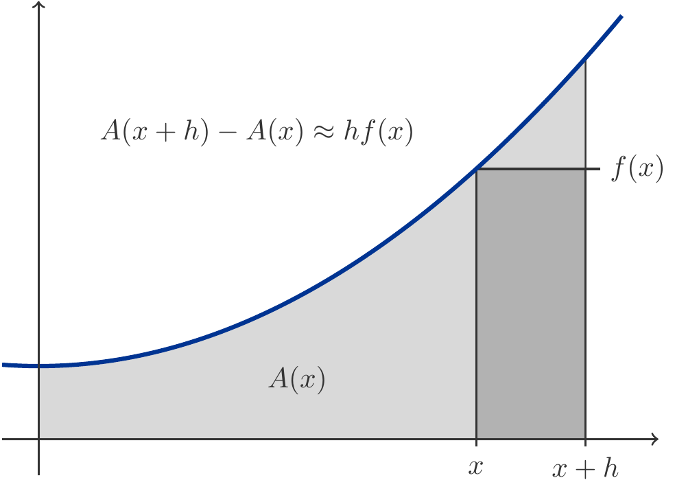
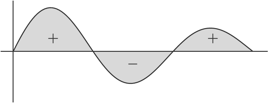
In summary: The (oriented) area under a function graph is identical to the definite integral of the function.
Exercise 4.25 Calculate the area under the function \(f(x)=e^{-2x}\) between the limits \(x=0\) and \(x=10\).
Solution: \[ \begin{gathered} \int_0^{10} e^{-2x}dx=-\frac{1}{2}e^{-2x}\Big|_0^{10}= -\frac{1}{2}e^{-20}+\frac{1}{2}\simeq 0.5 \end{gathered} \] □
4.3.2 Average Values
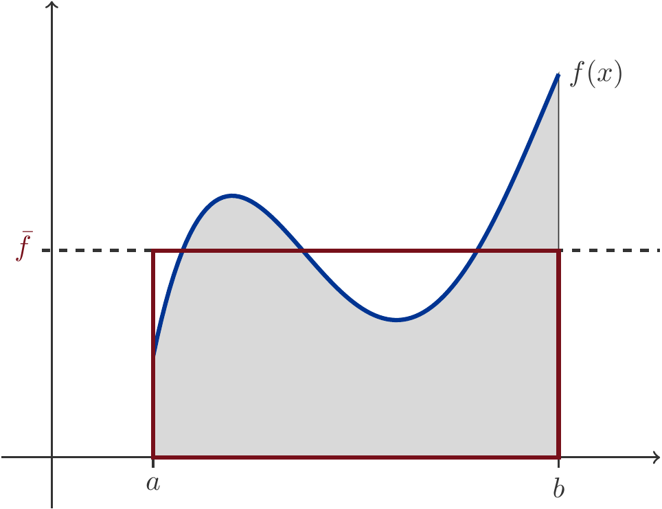
The average value \(\bar{f}\) of a function \(f\) over an interval \([a,b]\) is defined as the height of a rectangle over the interval that encloses the same area as the function graph. This means \[ \begin{gathered} \bar{f}(b-a)=\int_a^b f(x)\,dx\quad\implies\quad \bar{f}=\frac{1}{b-a} \int_a^b f(x)\,dx \end{gathered} \tag{4.10}\] The relation (4.10) is also called the mean value theorem of integral calculus.
Exercise 4.26
- Calculate the average value of \(f(x)=x\) over the interval \([0,5]\).
- Calculate the average value of \(f(x)=e^{-x}\) over the interval \([0,5]\).
Solution: \[ \begin{gathered} \frac{1}{5}\int_0^5 x\,dx=\frac{1}{5}\frac{x^2}{2}\Big|_0^5=2.5\\[4pt] \frac{1}{5}\int_0^5 e^{-x}\,dx=-\frac{e^{-x}}{5}\Big|_0^5=\frac{1-e^{-5}}{5}\Big|_0^5=0.1987\,. \end{gathered} \] □
In many applications, such as inventory theory or queuing theory, piecewise linear functions and their averages play an important role.
An example is the function \(f(x)\) defined by: \[ \begin{gathered} f(x)=\left\{\begin{array}{cl} 2 & 0\le x < 3\\ 4 & 3\le x < 6\\ 3 & 6\le x < 7\\ 5 & 7\le x < 9 \end{array}\right. \end{gathered} \] We can imagine that \(x\) represents the time and \(f(x)\) the number of customers waiting at time \(x\). What is then the average length of the queue?
The graph of the function \(f(x)\) is shown in Figure 4.6.
This function has discontinuities at \(x=3\), \(x=6\), and \(x=7\). Its average value \(\bar{f}\) is \[ \begin{gathered} \bar{f}=\frac{1}{9}\int_0^9f(x)\,\mathrm{d}x. \end{gathered} \]
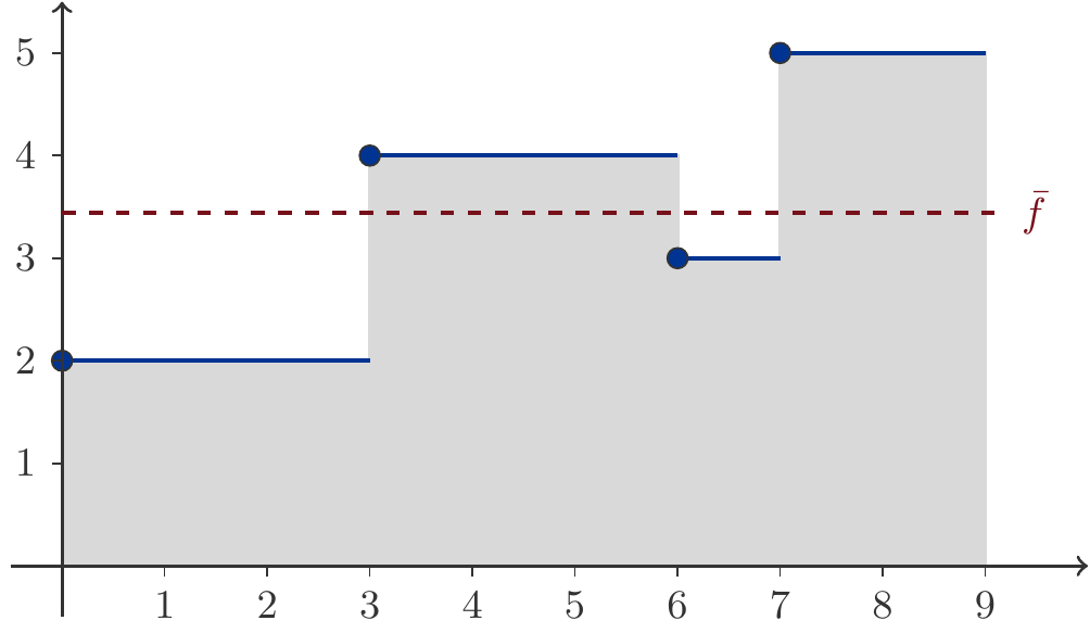
But how do we calculate this integral? For this, we use the additivity property from Theorem 4.6: \[ \begin{aligned} \bar{f}&=\frac{1}{9}\left[\int_0^32\,\mathrm{d}x+ \int_3^64\,\mathrm{d}x+\int_6^73\,\mathrm{d}x+\int_7^95\,\mathrm{d}x\right]=\\[5pt] &=\frac{1}{9}\left[2x\big|_0^3+4x\big|_3^6+3x\big|_6^7+5x\big|_7^9\right]\\ &=\frac{1}{9}\left[2\cdot 3+4\cdot(6-3)+3\cdot(7-6)+5\cdot(9-7)\right] =\frac{31}{9}\simeq 3.44\,. \end{aligned} \] If \(f(x)\) were to describe the length of a queue over the time interval \([0,9]\), then this queue would have an average length of 3.44 customers.
4.3.3 Inventory Management
In Chapter 3, we have already dealt with inventory management and derived the classical inventory formula for the simplest model, Economic Order Quantity, in a relatively informal way.
Let us recall that in this simple model, there are essentially three cost drivers: (a) the number of ordering processes per unit of time, (b) the acquisition costs of the stored goods, and (c) the average inventory level. In the EOQ model, the latter is exactly half the optimal order quantity \(x^\ast\) (see Figure 3.16).
We now want to clarify why we are allowed to argue that the costs of physical storage are proportional to the average inventory level.
The storage of a good costs \(h\) currency units per unit of time and unit of quantity. The inventory level is variable and is given by the function \(I(t)\). How can one calculate the costs for storage?
Let us denote the costs incurred for storage in the time interval \([0,t]\) by \(C(t)\). The inventory level typically changes over time, but for very small time intervals \([t,t+\epsilon]\), we can assume that the stored quantity \(I(t)\) remains approximately the same. Then the following approximations hold \[ \begin{gathered} C(t+\epsilon)-C(t)\approx hI(t)\epsilon\quad\text{or}\quad \frac{C(t+\epsilon)-C(t)}{\epsilon}\approx hI(t)\;. \end{gathered} \] For \(\epsilon\to 0\) we therefore have \[ \begin{gathered} C'(t)=hI(t), \end{gathered} \] implying that the storage costs are an antiderivative of the function \(hI(t)\), and therefore: \[ \begin{gathered} C(T)=h\int_0^T I(t)\,\mathrm{d}t. \end{gathered} \] Considering that because of the mean value theorem (4.10) \[ \begin{gathered} \bar{I}=\frac{1}{T}\int_0^T I(t)\,\mathrm{d}t \end{gathered} \] expresses the average inventory level, the formula for storage costs is \[ \begin{gathered} C(T)=hT\bar{I},\quad\text{for all }T\ge 0. \end{gathered} \] Thus, the storage costs can always be calculated by assuming a constant inventory at the level of the average inventory.
Exercise 4.28 In the time interval \((0,10)\), an inventory function \(I(t)\) is given by: \[ \begin{gathered} I(t)=\left\{\begin{array}{ll} -t+4 & 0\le t<3\\ -t+8 & 3\le t < 5\\ -t+12 & 5\le t< 10 \end{array}\right. \end{gathered} \] What is the average inventory level \(\bar{I}\)?
Solution: The function is quite similar to the one we have already encountered in fig-3-Lagerbestandsverlauf. Its graph is shown in Figure 4.7.
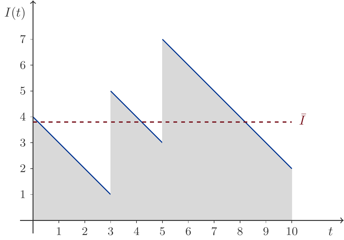
We calculate the average inventory level as follows: \[ \begin{aligned} \bar{I}&=\frac{1}{10}\left[\int_0^3(-t+4)\,\mathrm{d}t+\int_3^5(-t+8)\,\mathrm{d}t + \int_5^{10}(-t+12)\,\mathrm{d}t\right]\\[5pt] &=\frac{1}{10}\left[ \left(-\frac{t^2}{2}+4t\right)\bigg|_0^3 +\left(-\frac{t^2}{2}+8t\right)\bigg|_3^5 +\left(-\frac{t^2}{2}+12t\right)\bigg|_5^{10} \right]\\[5pt] &=3.8\,. \end{aligned} \]
Exercise 4.29
What is the average inventory level if the inventory height starts at \(L(0)=1000\), decreases uniformly (linearly) and ends at \(L(10)=500\)?
What is the average inventory level if the inventory height starts at \(L(0)=1000\), decreases at a constant relative rate and ends at \(L(10)=500\)?
Solution: (1) Linear decrease means \(L(t) = a-bt\) with \[ \begin{gathered} L(0)=1000,\quad L(10)=500\implies L(t)=1000-50t. \end{gathered} \] The average level is therefore: \[ \begin{gathered} \bar{L}=\frac{1}{10}\int_0^{10}(1000-50t)\,dt=750. \end{gathered} \]
(2) Decrease at a constant relative rate means \(L(t)=L(0)e^{-at}\) with \[ \begin{gathered} L(0)=1000, \quad L(10)=500\implies L(t) =1000e^{-0.0693 t}. \end{gathered} \] The average level now amounts to: \[ \begin{gathered} \bar{L}=\frac{1}{10}\int_0^{10}1000e^{-0.0693t}\,dt=721.35\,. \end{gathered} \] □
4.3.4 Continuous Cash Flows
We have already discussed the interpretation of definite integrals in connection with continuous cash flows.
Exercise 4.30 A capital of 1000 CU is increased at the rate of \(a(t)=3-0.1t\). How much is the capital after 10 periods?
Solution: From the problem statement, it follows that the capital’s rate of change \(K'(t)=a(t)=3-0.1t\). Therefore, due to (4.2): \[ \begin{aligned} K(10)&=K(0)+\int_0^{10} a(t)\,\mathrm{d}t=1000+\int_0^{10} (3-0.1t)\,\mathrm{d}t\\ &=1000+(3t-0.05t^2)\Big|_0^{10}=1000+30-5=1025. \end{aligned} \] □
Continuous cash flows typically are subject to compounding as in financial annuities.
Future Value and Present Value of Cash Flows
Let \(K(0)\) be a capital that is continuously compounded at the nominal interest rate \(c\) and to which new capital is added at the rate \(a(t)\). The designation \(a(t)\) for the capital inflow is not chosen at random. In Chapter 2 we referred to payments of an annuity with \(a\), which there were assumed to be constant. Now, we will more generally allow that payments depend explicitly on time.
We want to calculate the future value the capital has grown to after the time \(T\).
The capital’s rate of change due to interest alone would be \(K'(t)=cK(t)\), because the nominal interest rate is the relative rate of change of the capital, i.e., \(K'(t)/K(t)=c\). When we consider both sources of asset change, the total rate of change of the capital becomes: \[ \begin{gathered} K'(t)=cK(t)+a(t). \end{gathered} \tag{4.11}\] This is a differential equation. Such equations are generally extremely difficult to solve. Fortunately, we have a relatively simple situation here.
To find the unknown function \(K(t)\), we multiply both sides of (4.11) by the factor \(e^{-ct}\). In short, we discount, turning to present values. After rearranging, we discover something interesting: \[ \begin{gathered} \underbrace{e^{-ct}K'(t)-ce^{-ct}K(t)}_{(e^{-ct}K(t))'}=e^{-ct}a(t). \end{gathered} \] The left side results from applying the product rule to the present value of the capital \(e^{-ct}K(t)\): \[ \begin{gathered} \Big( e^{-ct}K(t)\Big)'=e^{-ct}a(t). \end{gathered} \] The right side is the present value of the payment at time \(t\). Thus, \(e^{-ct}K(t)\) is a primitive function of \(e^{-ct}a(t)\) and we can say: \[ \begin{gathered} e^{-cT}K(T)=K(0)+\int_0^T e^{-ct} a(t)\,\mathrm{d}t. \end{gathered} \tag{4.12}\] Indeed, this is a formula for the present value of a continuous annuity with initial capital \(K(0)\).
Aside from the initial value \(K(0)\), (4.12) is analogous to the present value formula (2.11) from Chapter 2: the present value of the cash flow is the sum of the discounted payments, where here sum means integral2.
If we compound (4.12), i.e., multiply both sides of this equation by the compounding factor \(e^{cT}\), then we get a future value formula: \[ \begin{gathered} K(T)=e^{cT}K(0)+\int_0^T e^{c(T-t)}a(t)\,\mathrm{d}t. \end{gathered} \tag{4.13}\] This formula is, aside from the initial capital, analogous to (2.13): the future value of a continuous cash flow results from the future value of the initial capital plus the (continuous) sum of payments compounded over the remaining term \(T-t\), \(e^{c(T-t)}a(t)\).
Exercise 4.31 What is the future value of a cash flow at a constant rate of \(a(t)=2000\) and an interest rate \(c=0.05\) after 10 years?
Solution: Since no initial capital is specified here, we may assume \(K(0)=0\). We now apply (4.13): \[ \begin{gathered} K(10)=\int_0^{10}e^{0.05(10-t)}2000\,\mathrm{d}t =2000e^{0.5}\int_0^{10}e^{-0.05t}\,\mathrm{d}t =25948.85\,. \end{gathered} \] But the last integral is very simple to calculate using Theorem 4.19: \[ \begin{gathered} \int_0^Te^{-ct}\,\mathrm{d}t=-\frac{1}{c}\,e^{-ct}\bigg|_0^T=\frac{1-e^{-cT}}{c}\,. \end{gathered} \tag{4.14}\] In our example: \[ \begin{gathered} \int_0^{10}e^{-0.05t}\,\mathrm{d}t=\frac{1-e^{-0.05\cdot 10}}{0.05}=7.86938681, \end{gathered} \] and therefore: \[ \begin{gathered} K(10)=2000\cdot e^{0.5}\cdot 7.86938681=25948.85085\simeq 25949. \end{gathered} \] □
Exercise 4.32 What constant payment stream \(a\) must be added to a savings account so that it reaches the amount of 10000 CU after 8 years (nominal interest rate 4 percent)?
Solution: We apply the future value formula (4.13) with \(K(0)=0\). Then the payment stream \(a\) must produce the future value \[ \begin{gathered} 10000=\int_0^8 e^{0.04(8-t)}a\,\mathrm{d}t = a\cdot e^{0.32}\int_0^8e^{-0.04t}\,\mathrm{d}t \end{gathered} \] We calculate the integral using (4.14): \[ \begin{gathered} \int_0^8e^{-0.04t}\,\mathrm{d}t=\frac{1-e^{-0.04\cdot 8}}{0.04}=6.84627407\,. \end{gathered} \] Therefore, \[ \begin{gathered} a=\frac{10000}{e^{0.32}\cdot 6.84627407}=1060.648507\simeq 1061\,. \end{gathered} \] □
Exercise 4.33 How high must a constant repayment rate be to repay a debt of 50000 CU after 10 years (nominal interest rate 5 percent)?
Solution: The constant repayment rate \(a\) must result in the future value \[ \begin{gathered} 0=50000e^{0.05\cdot10}+\int_0^{10} e^{0.05(10-t)}(-a)\,\mathrm{d}t \end{gathered} \] By dividing through the compounding factor \(e^{0.05\cdot10}\), thus switching to present values, we obtain the simpler equation: \[ \begin{gathered} 0=50000-a\int_0^{10} e^{-0.05t}\,\mathrm{d}t. \end{gathered} \] The integral has already been calculated in the solution to Exercise 4.31: \[ \begin{gathered} a=\frac{50000}{7.86938681}=6353.735205\simeq 6354. \end{gathered} \] □
Exercise 4.34 How high must an initially constant repayment rate that gradually decreases to zero be in order to repay a debt of 50000 CU after 10 years (nominal interest rate 5 percent)?
Solution: If the repayment rate \(a(t)\) with initial value \(a_0\) decreases uniformly, i.e., linearly, to zero over 10 years, then \(a(t)\) must satisfy the equation: \[ \begin{gathered} a(t)=a_0\left(1-\frac{t}{10}\right). \end{gathered} \] This repayment rate must produce the end value \[ \begin{gathered} 0=50000e^{0.05\cdot10}-\int_0^{10} e^{0.05(10-t)}a_0\left(1-\frac{t}{10}\right)\,\mathrm{d}t \end{gathered} \] By dividing again by the compounding factor, i.e., moving to present values, we obtain: \[ \begin{gathered} 0=50000-a_0\int_0^{10} e^{-0.05t}\left(1-\frac{t}{10}\right)\,\mathrm{d}t, \end{gathered} \] this provides the initial value of the repayment rate: \[ \begin{gathered} a_0=\frac{50000}{\int_0^{10} e^{-0.05t}\left(1-\frac{t}{10}\right)\,\mathrm{d}t }\,. \end{gathered} \] The integral on the right side now requires some more effort. We break it up into two parts: \[ \begin{aligned} I&=\int_0^{10} e^{-0.05t}\left(1-\frac{t}{10}\right)\,\mathrm{d}t\\[5pt] &=\int_0^{10}e^{-0.05t}\,\mathrm{d}t-\frac{1}{10}\int_0^{10} t\cdot e^{-0.05t}\,\mathrm{d}t. \end{aligned} \] We have computed the first integral several times in the last exercises, its value is specifically \(7.86938681\), but generally (4.14). The second integral we have to compute using partial integration (Theorem 4.13): \[ \begin{gathered} \int_0^T t\cdot e^{-ct}\,\mathrm{d}t=\frac{-(1+ct)e^{-ct}}{c^2}\bigg|_0^T=\frac{1-(1+cT)e^{-cT}}{c^2}\,. \end{gathered} \] From this, we calculate for the current task: \[ \begin{gathered} \int_0^{10}t\cdot e^{-0.05t}\,\mathrm{d}t=\frac{1-(1+0.05\cdot 10)e^{-0.05\cdot 10}}{0.05^2}=36.0816042\,. \end{gathered} \] Therefore, we have \[ \begin{gathered} I=7.86938681-\frac{36.0816042}{10}= 4.26122639\,. \end{gathered} \] This finally gives us the initial value \(a_0\) of the repayment rate: \[ \begin{gathered} a_0=\frac{50000}{\int_0^{10} e^{-0.05t}(1-t/10)\,dt} = \frac{50000}{4.26122639}= 11733.71124. \end{gathered} \] □
4.4 Additional Exercises
-
Determine for \[ \begin{gathered} f(x)=3x^3-20x^2+5x-10 \end{gathered} \] an antiderivative \(F(x)\) such that \(F(0)=38\). What value does \(F(6)\) have?
Solution: \(F(6)=-400\).
-
A company produces with marginal costs \[ \begin{gathered} C'(x)=3x^2-6x+14,\quad x=\text{ Output}. \end{gathered} \] At an output of 10 units, the total costs amount to 2840 U. How high are the total costs at an output of 20 units?
Solution: \(C(20)=9080\)
-
Calculate \(I=\int_1^2 f(x)\,\mathrm{d}x\) with \(\displaystyle f(x)=-3x^2+5+\frac{4}{x^2}\).
Solution: Antiderivative \(\displaystyle F(x)=-x^3+5x-\frac{4}{x}+C\), \(I=0\).
-
Calculate \(I=\int_0^2 f(x)\,\mathrm{d}x\) with \(\displaystyle f(x)=e^{5x-9}\).
Solution: Antiderivative \(\displaystyle F(x)=\frac{1}{5}e^{5x-9}+C\), \(I=0.5436\).
-
Calculate \(I=\int_1^5 f(x)\,\mathrm{d}x\) with \(\displaystyle f(x)=\frac{4}{2x+5}\).
Solution: Antiderivative \(F(x)=2\ln(2x+5)+C\), \(I=1.5243\).
-
Calculate \(I=\int_0^1 f(x)\,\mathrm{d}x\) with \(\displaystyle f(x)=5xe^{-4x^2}\).
Solution: Antiderivative \(\displaystyle F(x)=-\frac{5}{8}e^{-4x^2}+C\), \(I=0.6136\).
-
Calculate \(I=\int_1^4 f(x)\,\mathrm{d}x\) with \(f(x)=\ln(x^2)\).
Solution: Antiderivative \(F(x)=2x(\ln x-1)+C\), \(I=5.0904\).
-
Calculate \(I=\int_{-1}^1 f(x)\,\mathrm{d}x\) with \(\displaystyle f(x)=\frac{12x}{5+2x^2}\).
Solution: Antiderivative \(F(x)=3\ln(5+2x^2)+C\), \(I=0\).
-
Calculate \(I=\int_{1}^2 f(x)\,\mathrm{d}x\) with \(f(x)=(2x+1)\sqrt{x^2+x+1}\).
Solution: Antiderivative \(\displaystyle F(x)=\frac{2}{3}(x^2+x+1)^{3/2}+C\), \(I=8.8827\) .
-
Calculate \(I=\int_{0}^2 f(x)\,\mathrm{d}x\) with \(f(x)=xe^{-2x}\).
Solution: Antiderivative \(\displaystyle F(x)=-\frac{1}{4}(2x+1)e^{-2x}+C\), \(I=0.2271\) .
-
Calculate \(I=\int_{1}^{10} f(x)\,\mathrm{d}x\) with \(f(x)=x^2\ln x\).
Solution: Antiderivative \(\displaystyle F(x)=\frac{x^3}{9}\left(3\ln x-1\right)+C\), \(I=656.5284\) .
-
Calculate \(I=\int_{0}^{1} f(x)\,\mathrm{d}x\) with \(f(x)=\sqrt{e^{4x}}\).
Solution: Antiderivative \(\displaystyle F(x)=\frac{1}{2}e^{2x}+C\), \(I=3.1945\) .
-
What is the average value of the function \(f(x)=x^2-2x+5\) in the interval \((-1,1)\)?
Solution: \(\bar{f}=16/3\).
-
What is the average value of the function \(f(x)=e^{-x/4}\) in the interval \((1,10)\)?
Solution: \(\bar{f}=0.3097\).
-
What is the average value of the function \(f(x)=\ln x\) in the interval \((1,100)\)?
Solution: \(\bar{f}=3.6517\).
-
What is the average inventory level if the inventory height starts at \(L(0)=4046\), decreases uniformly (linearly) and ends at \(L(16)=2354\)?
Solution: \(\bar{I}=3200\).
-
What is the average inventory level if the inventory height starts at \(L(0)=6556\), decreases at a constant relative rate and ends at \(L(8)=1423\)? Round the result to a whole number.
Solution: \(\bar{I}=3360\).
-
An inventory level function is given by: \[ \begin{gathered} I(t)=\left\{\begin{array}{cl} 3 & 0\le t< 2\\ 5 & 2\le t < 5\\ 2 & 5\le t<8 \end{array}\right. \end{gathered} \] Calculate the average inventory level.
Solution: \(\bar{I}=27/8=3.375\)
-
An inventory level function is given by: \[ \begin{gathered} I(t)=\left\{\begin{array}{cl} -\frac{t}{2}+2 & 0\le t< 2\\[4pt] -\frac{t}{2}+4 & 2\le t < 3 \end{array}\right. \end{gathered} \] Calculate the average inventory level.
Solution: \(\bar{I}=23/12=1.92\)
-
A capital amount of 2000 CU is increased at the rate \(a(t)=11-0.14t\). What is the capital after 35 periods? Round the result to a whole number.
Solution: 2299.25 CU
-
What is the final value of a payment stream at constant rate \(a(t)=3300\) with an interest rate \(c=0.09\) after 4 years? Round the result to a whole number.
Solution: 15889 CU
-
What constant payment stream is required to reach a savings balance of 14900 CU after 7 years. Calculate with a nominal interest rate of 10 percent and round the result to a whole number.
Solution: 1470 CU
-
How high must a constant amortization rate be to repay a debt of 19000 CU after 5 years? Calculate with a nominal interest rate of 6 percent and round the result to a whole number.
Solution: 4398 CU
-
How high must an amortization rate that decreases uniformly to zero initially be to repay a debt of 11000 CU after 6 years? Calculate with a nominal interest rate of 6 percent and round the result to a whole number.
Solution: 4120 CU