1 Linear and Quadratic Functions
1.1 Linear Functions
Among real functions, the simplest are the linear ones. However, their importance is not solely due to their simplicity. Linear functions are often used to approximate more complicated functions.
1.1.1 Function Terms
Definition 1.1 Functions \(f:\mathbb R \rightarrow \mathbb R\) with a function term in the form of \(f(x)=kx\) or \(f(x)=kx+d\) are called linear functions.
A linear function has as its domain the set \(\mathbb R\) of all real numbers. We distinguish between homogeneous linear functions with the function term \(f(x)=kx\) and inhomogeneous linear functions with a function term \(f(x)=kx+d\), where \(d\not=0\).
The function terms \(f(x)=3x\), \(g(x)=-0.5x\), \(h(x)=4.37x\) define homogeneous linear functions. The function term \(s(x)=-7x+2\) defines an inhomogeneous linear function.
1.1.2 Graphs of Functions
What does the graph of linear functions look like? What is special about the graphs of linear functions? It will be found that the graphs of linear functions are characterized by a straight-line trajectory.
But what does straight-line mean? Intuitively, this is completely clear, but what is the mathematical expression of straight-line in the function term of a linear function? To answer these questions, let us recall the concept of slope.
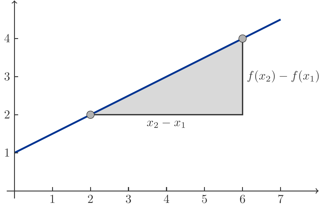
Remark 1.3 (Slope) Let us first consider a totally arbitrary real function \(f\). Let \(x_1\) and \(x_2\) be two points in the domain and \(f(x_1)\) and \(f(x_2)\) be the values of the function at these points. How much does the function \(f\) change as the variable \(x\) goes from \(x_1\) to \(x_2\)?
An initial response consists of indicating the difference \(f(x_2)-f(x_1)\). That, indeed, is the change in the function values between \(x_1\) and \(x_2\). However, this size is not a very interesting measure of the strength of the change, as the difference naturally also depends on the step size \(x_2-x_1\). To fairly compare the changes of the function with large and small steps, we should rather use the average change \[ \begin{gathered} \frac{f(x_2)-f(x_1)}{x_2-x_1} \end{gathered} \] This average change is also called the slope or the difference quotient of the function between \(x_1\) and \(x_2\). With an arbitrary real function, this slope can of course change when one alters the points \(x_1\) and \(x_2\).

Now let \(f(x)=kx+d\) be a linear function. If one takes any two numbers \(x_1\) and \(x_2\) from the domain and calculates the slope between these points, one obtains (cf. Figure 1.1) \[ \begin{gathered} \frac{f(x_2)-f(x_1)}{x_2-x_1}=\frac{(kx_2+d)-(kx_1+d)}{x_2-x_1}=k. \end{gathered} \tag{1.1}\]
This equation means that the slope of the graph of a linear function is always the same, regardless of the choice of \(x_1\) and \(x_2\). This property is visually expressed in the graph by its straight-line trajectory. The constant slope is the mathematical characteristic responsible for the straight-line course.
A linear function \(f(x)=kx+d\) has two parameters, \(k\) and \(d\), both of which influence the geometric appearance of the function graph. As already known from (1.1), the parameter \(k\) indicates the slope, shortly the gradient, of the function graph. The geometric meaning of the parameter \(d\) is just as easy to see. It is \(f(0)=k\cdot 0 +d=d\). Thus, \(d\) is the function value at the point \(x=0\). In other words, the graph of the linear function \(f(x)=kx+d\) intersects the vertical coordinate axis at the point \((0,d)\).
Remark 1.4 (Equations of Lines) As a result of our considerations, we have seen that the graph of a linear function is always a straight line. However, the converse is not true! Not every straight line is the graph of a linear function. There are also lines that run vertically. Such lines do not have a slope ratio and therefore cannot be the graphs of linear functions.
Arbitrary lines are described in a coordinate system by linear equations of the form \(ax+by+c=0\). A general line is a set of points of the form \[ \begin{gathered} g=\{(x,y): ax+by+c=0\}. \end{gathered} \]
If \(b\ne 0\), then the line \(g\) is a graph of a function. We can calculate \(f(x):=y=-\frac{a}{b}x-\frac{c}{b}\), the so-called standard form, and see that \[ \begin{gathered} g=\{(x,y): ax+by+c=0\}=\{(x,y): y=f(x)\}, \end{gathered} \]
so \(g\) is the graph of a linear function. But if \(b=0\), the equation \(ax+c=0\) does not define a function, because it must then be that \(x=-\frac{c}{a}\) is constant and \(y\) can take any arbitrary value. Therefore, every pair \((-\frac{c}{a},y)\) with an arbitrary \(y\in\mathbb R\) satisfies the equation and the corresponding point lies on the line, which now runs vertically. Such lines cannot appear as graphs of functions.
Remark 1.5 (Calculation of the Parameters \(k\) and \(d\)) As many examples in this chapter will show, it is a recurring task to calculate the parameters \(k\) and \(d\) from suitable information. A typical situation is as follows: two points \(P=(x_0,y_0)\) and \(Q=(x_1,y_1)\) are given, whose coordinates satisfy the function equation \(y=kx+d\) of a linear function, with \(k\) and \(d\) unknown. Geometrically, the graph of the function runs through both points \(P\) and \(Q\).
Here’s how we proceed: \(k\) is the slope ratio, so: \[ \begin{gathered} k=\frac{y_1-y_0}{x_1-x_0}=\frac{\Delta y}{\Delta x}, \end{gathered} \tag{1.2}\]
From the equation \(y=kx+d\), \(d\) follows immediately when we substitute the point \(P\) or \(Q\): \[ \begin{aligned} d &= y_0-k x_0=y_1-kx_1. \end{aligned} \tag{1.3}\]
Exercise 1.6 Determine the function equation of the linear function whose graph passes through the points \(P=(3,8)\) and \(Q=(7,4)\).
Solution: From (1.2) and (1.3) we get: \[ \begin{gathered} k=\frac{4-8}{7-3}=-1,\quad d=8-(-1)\cdot 3=11\;. \end{gathered} \] Therefore, \(y=-x+11\). □
1.1.3 Costs and Revenues
We will now discuss some economic applications of linear functions. In these examples, it turns out that the mathematically possible domain of a linear function is usually not identical to the domain on which the function has an economically sensible interpretation. Usually, only nonnegative values \(x\ge 0\) make sense in an economic context.
Linear Cost Functions
In many areas, costs arise that are a linear function of the consumed quantity of some resources.
The costs a household has to pay for the consumption of electric power are a linear function of the consumed amount of electricity (measured in kilowatt-hours). This linear cost function \(C(x)=kx+d\) is composed of the basic charge \(d\), the tariff price \(k\) per kilowatt-hour and the consumed quantity \(x\).
For someone who does not have a contract with a generous flat rate, the phone costs per month are a linear function of the consumed minutes of conversation. This linear cost function \(C(x)=kx+d\) is composed of the monthly basic fee \(d\), the tariff price \(k\) per minute and the number \(x\) of conversation minutes per month.
Even in the production of goods, linear cost functions are a simple, yet important mathematical model. Let \(C(x)=kx+d\) be any linear cost function, where \(x\) indicates the quantity of goods produced. Then \(C(0)=d\) are the fixed costs, which occur even when no production is taking place. The variable costs therefore amount to \(V(x)=C(x)-C(0)=kx\). These are the quantity-dependent costs.
What are the production costs of a unit quantity (unit costs) when a linear cost function is present?
This question has two different answers depending on what one understands by the production costs of a unit quantity. One possible interpretation understands the unit costs to be the average costs \[ \begin{gathered} \overline{C}(x)=\frac{C(x)}{x}, \end{gathered} \] which are caused by the production of one unit of quantity. For a linear cost function, the average costs are \[ \begin{gathered} \overline{C}(x)=\frac{C(x)}{x}=\frac{kx+d}{x}=k+\frac{d}{x}. \end{gathered} \] However, \(\overline{C}(x)\) is no longer a linear function (see Figure 1.2).
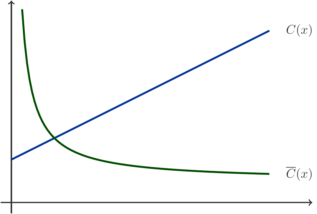
Thus, the average costs also include a share of the fixed costs \(d/x\), which becomes smaller as the quantity \(x\) increases.
Another possible interpretation of unit costs refers to the costs incurred by the production of an additional unit quantity. So, if we produce the quantity \(x\) and want to produce one more unit, this causes additional costs equal to \(C(x+1)-C(x)\). These additional costs of an extra unit quantity are also known as marginal costs. The marginal costs for a linear cost function are \[ \begin{gathered} C(x+1)-C(x)=k(x+1)+d-(kx+d)=k. \end{gathered} \] In the linear cost model, the marginal costs are therefore independent of how much is currently being produced. It does not matter whether little or much is produced, the marginal costs of an additional piece always amount to the same. With higher production, the average costs decrease, while the marginal costs always remain the same.
Let’s now look at a numerical example.
Exercise 1.7 The cost function is given by \(C(x)=5x+3000\). The current production is \(x=10\,000\) units. What are the average unit costs and what are the marginal costs?
Solution: The average costs amount to \[ \begin{gathered} \overline{C}(10000)=\frac{C(10000)}{10000}=\frac{5\cdot 10000+3000}{10000}=5.3\;. \end{gathered} \] In contrast, the marginal costs amount exactly to \(5\). □
The characteristic of constant marginal costs is indicative of a linear cost function. It also shows the limitations of the linear cost model in practice. The trajectory of marginal costs is usually not constant.
Revenue Functions
Let the sales price of a unit of a good be \(p\). We denote the sold quantity by \(x\). Then the revenue (English: revenue), which is achieved from the sale of quantity \(x\), is \[ \begin{gathered} R(x)=px. \end{gathered} \] Hence, the revenue is a homogeneous linear function. The graph of the function is a straight line that passes through the point \((0,0)\) and has the slope \(p\).
The fact that the price is a given constant for market participants is typical for the market model of perfect competition, also known as polypoly. In microeconomics, this refers to a market in which many suppliers face many demanders, so many in fact, that none of the market participants have sufficient market power to influence the market price significantly through autonomous actions. On a monopoly market, however, the circumstances are entirely different, as we will see in Section 1.2.2.
Profitability in the Linear Cost Model
Let \(C(x)=kx+d\) be a linear cost function and \(R(x)=px\) be the revenue function. Production is profitable if the revenue exceeds the costs, i.e., if \(R(x)>C(x)\). In the case that \(R(x)<C(x)\), the production is unprofitable. It is important to know the profitability range, i.e., the set of all profitable production quantities \(x\ge 0\).
The profitability condition is \(R(x)>C(x)\), i.e. \(px>kx+d\) or \[ \begin{gathered} (p-k)x>d. \end{gathered} \] The difference \(p-k\) between the price and the marginal unit costs is called the contribution margin that can be achieved with the product. The fixed costs \(d\) are certainly non-negative, and the production quantities \(x\) are only meaningful as non-negative numbers. The profitability condition can only be met if the contribution margin \(p-k>0\) is positive, i.e., if \(p>k\). The condition is also economically clear, as profitable production is only possible if the achievable price of the goods exceeds the unit costs.
But even if \(p>k\), not every production quantity is profitable. The profitability condition \((p-k)x>d\) states that the quantity \(x\) must be at least large enough that the fixed costs \(d\) are compensated by \((p-k)x\) at least. This minimum quantity, at which a compensation of the fixed costs occurs, is therefore obtained by solving the equation \((p-k)x=d\), and it is: \[ \begin{gathered} x_0=\frac{d}{p-k}=\frac{\text{Fixed costs}}{\text{Contribution margin}}. \end{gathered} \] This is the break-even point or break-even threshold.
In general, one obtains the break-even point \(x_0\) computationally by solving the equation \(R(x)=C(x)\). The resulting profitability range is then \(\{x:\;x>x_0\}=(x_0,\infty)\).
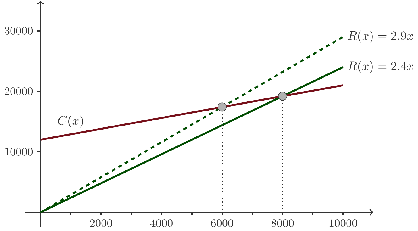
Exercise 1.8 The private brewery Naturgold is planning the introduction of a new product, a strong beer, which will be marketed under the name Favoritner Black Bock. According to the planning, the weekly fixed costs of production will amount to 12,000 GE. The variable costs per bottle of Black Bock are 0.9 GE, and the sales price is set at 2.4 GE per bottle.
What is the break-even point?
At what price would have to be set so that the break-even is reached at 6,000 bottles?
Solution: From the text of the statement, we infer the variable cost per bottle \(k=0.9\) and the fixed costs \(d=12,000\). Therefore, the cost function is: \(C(x) = 0.9x + 12,000\). The revenue function is \(R(x)=p\cdot x=2.4x\). The profit function is then derived as \[ \begin{gathered} \pi(x) = R(x) - C(x)= 2.4x - (0.9x + 12,000) = 1.5x - 12,000. \end{gathered} \] We calculate the break-even point by equating revenue and costs: \[ \begin{aligned} R(x) = C(x)\quad\Rightarrow&\quad& 2.4x =&\; 0.9x + 12,000\\[4pt] \quad\Rightarrow&\quad &x=&\; \frac{12,000}{2.4-0.9}=8000\;\text{bottles per week}. \end{aligned} \] If break-even should be reached at \(x=6000\) bottles per week, then this requires a selling price \(p\): \[ \begin{gathered} 6000=\frac{12,000}{p-0.9}\implies p-0.9=2\implies p=2.9. \end{gathered} \] □
Exercise 1.9 A company calculates the production cost of a new product at \(45\) CU (currency units) per unit. The one-time fixed costs for acquiring production machinery amount to \(15,000\) CU. \(250\) units of the product can be produced per month. How should the price per unit be set if the company aims to generate a profit of \(40,000\) CU after four months?
Solution: The cost function is \(C(x)=45x+15000\), the revenue function is \(R(x)=px\). We denote the profit achieved with a sales quantity of \(x\) units by \(\pi(x)=R(x)-C(x)\). The desired profit should be reached after 4 months, which with \(x=1000\) units. This means \[ \begin{aligned} \pi(1000)=40000&=R(1000)-C(1000)\\ &=1000p-(45\cdot 1000+15000)\\ &=1000p - 60000. \end{aligned} \] Thus, the price must be \(p=100\). □
Exercise 1.10 A company is planning to launch a new product, for which \(60,000\) CU (currency units) have been budgeted as fixed costs. The production of one unit incurs costs of \(150\) CU. The break-even point should be reached at 1200 units. Due to a patent dispute, production must be stopped after 300 units. What damage has been done to the company as a result?
Solution: The cost function is \(C(x)=150x+60,000\). For the quantity \(x=1200\) to correspond to the break-even point, \(C(x)=R(x)\) must hold true, i.e., \[ \begin{gathered} 150\cdot 1200 + 60,000 = p\cdot 1200 \implies 1200p = 240,000. \end{gathered} \] From this, the necessary price comes out as \(p=200\). If sales are stopped at \(x=300\), then the damage is \[ \begin{gathered} C(300) - R(300) = 150\cdot 300 + 60,000 - 200\cdot 300 = 45,000. \end{gathered} \] □
Exercise 1.11 A transport entrepreneur purchases a new truck for \(784,000\) monetary units (MU). The fixed annual costs, which include the repayment installments for the purchase, amount to \(25\%\) of the acquisition costs. When the truck is used, personnel costs of \(480\) MU per operating day and fuel costs of \(590\) MU per operating day arise. Each day, \(8\) transports can be carried out with the truck; the revenue per transport is \(440\) MU. After how many days of operation within a business year does the use of the truck become cost-effective?
Solution: First, we formulate the cost function \(C(x)\), where \(C(x)\) represents the costs that arise from operating the truck for \(x\) days: \[ \begin{gathered} C(x)=480x+590x+784,000 \cdot 0.25=1070x+196,000.\end{gathered} \] Then, we establish the revenue function \(R(x)\), where \(R(x)\) represents the revenue generated from operating the truck for \(x\) days: \[ \begin{gathered} R(x)=8 \cdot 440 \cdot x=3520x.\end{gathered} \] To calculate the break-even point, we set revenue equal to costs: \[ \begin{gathered} C(x)=R(x) \quad \Rightarrow \quad 1070x+196,000=3520x \quad \Rightarrow \quad x=80 \; \text{days}.\end{gathered} \] □
1.2 Quadratic Functions
In addition to linear functions, quadratic functions form another simple but very important class of real functions.
1.2.1 Function Terms
Definition 1.12 A quadratic function refers to a real function with a function term of the form \[ \begin{gathered} f(x)=ax^2+bx+c.\end{gathered} \tag{1.4}\]
Clearly, linear functions are special cases of quadratic functions, namely when \(a=0\). Therefore, we assume in the following that \(a \neq 0\). While the graph of a linear function is a straight line, there is a much wider variety of shapes for quadratic functions: their graph is a parabola (see Figure 1.4).
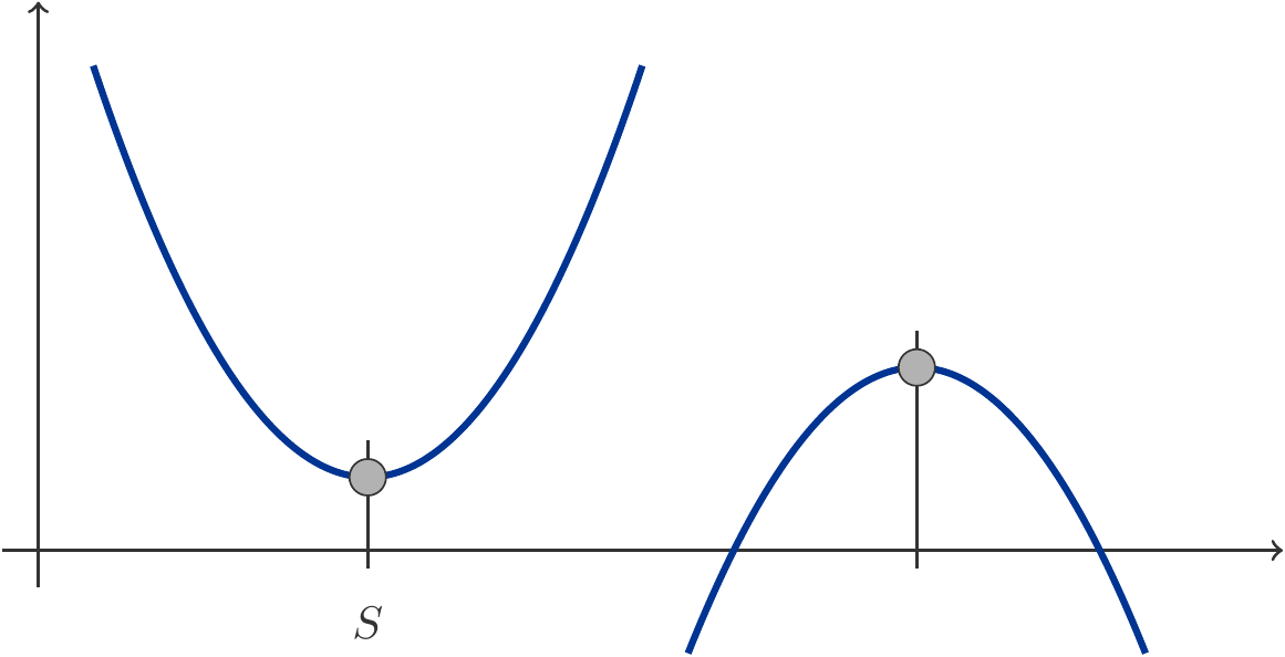
If \(a>0\), the parabola opens upward (also called convex), and the function takes on its minimum at the vertex \(x=S\). If \(a<0\), the parabola opens downward (concave), and the vertex is the maximum of the function. The position of the vertex can be easily determined by the well-known vertex formula: \[ \begin{gathered} S= -\frac{b}{2a}.\end{gathered} \tag{1.5}\]
Exercise 1.13 Determine the vertex of the quadratic function \(f(x)=2x^2-4x+7\).
Solution: We have \(a=2\) and \(b=-4\). Therefore, the \(x\)-coordinate of the vertex \(S\) is \(-b/2a=4/(2 \cdot 2)=1\). To calculate the \(y\)-coordinate, we simply substitute the \(x\)-coordinate into the function term: \[ \begin{gathered} f(1)=2\cdot1^2-4\cdot1+7=5. \end{gathered} \] Thus, \((1,5)\) is the vertex of \(f(x)\). □
1.2.2 Linear Market Model (Monopoly)
In this section, we will learn about typical applications where the analysis of a quadratic function is central. It is about the revenue and profit optimization of a monopolist. We base our considerations on a linear cost function and a linear demand function. The problem of profit optimization then leads to a quadratic function.
Revenue Optimization
A monopolist is a supplier who is the sole provider of his product on the market. He can freely choose the price of his product. In doing so, he controls the demand for his product.
Suppose the market’s demand function is \(D(p)=-ap+\alpha\). If the monopolist sets the price \(p\), his revenue is \[ \begin{gathered} R(p) = p \cdot D(p) = -ap^2 + \alpha p.\end{gathered} \] The revenue, therefore, is a quadratic function of the price, whose vertex is a maximum. To maximize revenue, the monopolist must choose the price \(p\) such that it exactly corresponds to the vertex of \(R(p)\).
Let’s look at an example.
Exercise 1.14 The operator of a ski lift, who has a local monopoly in a beautiful skiing area, had been able to sell 750 day passes a day at a price of 45 MU each two years ago. When he reduced the price to 40 MU per ticket last year, the sales increased to 800 tickets per day. At what ticket price does he achieve the highest daily revenue?
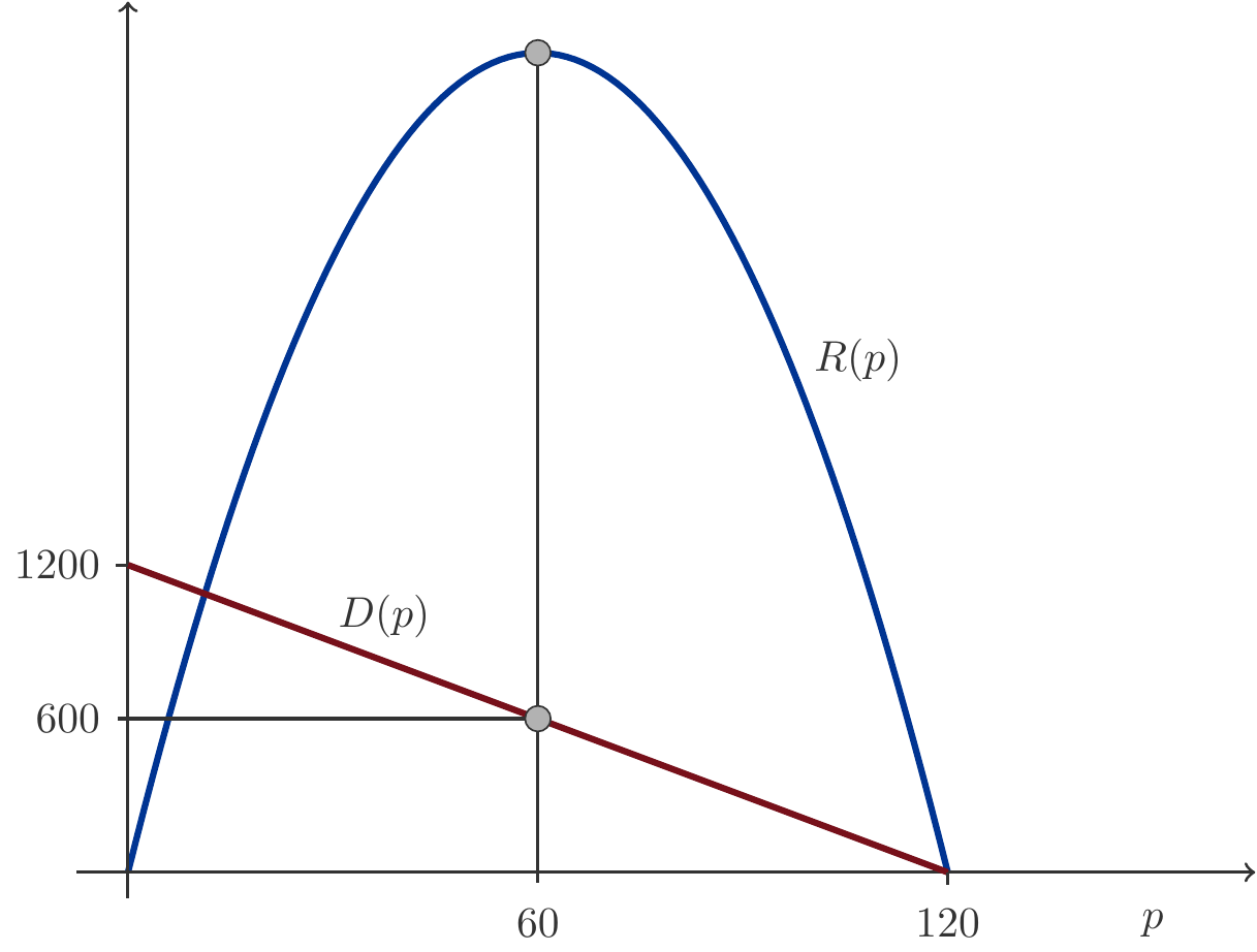
Solution: To determine the revenue function \(R(p) = p\cdot D(p)\) we first need the demand function \(D(p) = -ap+\alpha\). It passes through the points \(P=(45,750)\) and \(Q=(40,800)\). We calculate the parameters \(a\) and \(\alpha\) using (1.2) and (1.3): \[ \begin{gathered} \text{Slope }=-a=\frac{\Delta q}{\Delta p}=\frac{800-750}{40-45}=-10\implies a=10\\ \text{with point }P:\quad\alpha=D(p)+ap\implies \alpha=750+45\cdot 10=1200. \end{gathered} \] Thus we obtain \(D(p) = -10p+1200\). This gives us the revenue function: \[ \begin{gathered} R(p) = -10p^{2}+1200p \end{gathered} \] The vertex of this quadratic function is at \[ \begin{gathered} p_{\max} = -\dfrac{1200}{2\cdot (-10)} = 60.\end{gathered} \] Therefore, the maximum revenue is achieved at a price of \(60\) CU (currency units) per ski pass.
We will answer a few more questions.
What would the demand be then? \[ \begin{gathered} D(p_{\max}) = D(60) = -10\cdot 60 + 1200 = 600.\end{gathered} \] So, at this price \(600\) tickets will be demanded.
At what price does the demand disappear? \[ \begin{gathered} D(p) = 0 \quad\Rightarrow\quad -10p+1200 = 0 \quad\Rightarrow\quad p = 120.\end{gathered} \] This \(p\) is also called the prohibitive price.
Figure 1.5 illustrates our calculation.
Exercise 1.15 A dance school offers partner courses priced at 5260 CU per person. An increase in price by 460 CU results in the loss of one couple. At a price of 10580 CU per person, there are no more interested parties. At which price does the dance school achieve its highest revenue?
Solution: Let \(q\) be the number of persons participating in the course. From the information given, we deduce two points that the demand function must pass through: \(P(10580,0)\) and \(Q(10120,2)\), since if the prohibitive price of 10580 were reduced by 460, we would have one more couple, i.e. two more participants. Using (1.2) and (1.3), where \(k=-a\) and \(d=\alpha\): \[ \begin{gathered} k=-a=\frac{2-0}{10120-10580}=-\frac{1}{230}\implies a=\frac{1}{230},\\[5pt] d=\alpha=0-\left(-\frac{1}{230}\right)\cdot 10580=46\implies \alpha =46.\end{gathered} \] Thus the demand function is: \[ \begin{gathered} D(p) = -\frac{p}{230}+46,\end{gathered} \] and the revenue function is: \[ \begin{gathered} R(p) = -\frac{p^2}{230}+46p.\end{gathered} \] Its vertex is at \[ \begin{gathered} p_{\max} = -\frac{46}{-2/230}=5290.\end{gathered} \] In other words, the highest revenue is achieved at a price of 5,290 CU per person.
How many people will participate in the dance course at this price setting? \[ \begin{gathered} D(p_{\max}) = D(5290) = -\dfrac{1}{230}\cdot 5290 + 46=23\text{ people}.\end{gathered} \] 11–12 couples, meaning 23/2 individuals, will attend the dance course. □
Profit Optimization
In this section we learn through concrete examples how the problem of profit optimization for simple monopoly and competitive markets with linear or quadratic cost functions can be solved using elementary tools. However, in the case of more complex cost functions, we rely on methods of calculus, which we will discuss in Chapter 3.
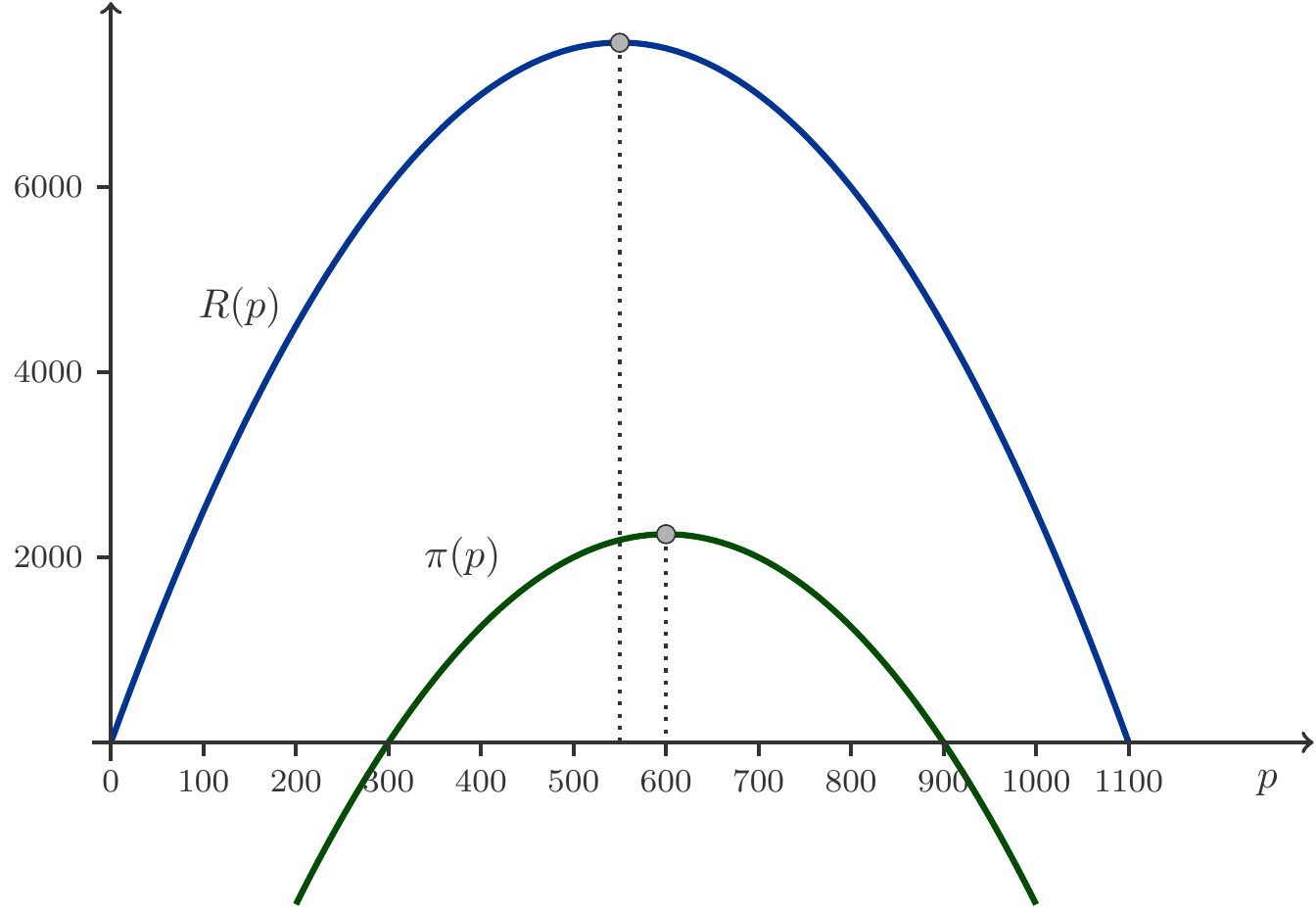
A lodging business has fixed daily costs of 8000 CU (currency units). The variable costs per bed amount to 100 CU. If \(q\) equals the number of occupied beds, then the cost function is \[ \begin{gathered} C(q)=100q+8000.\end{gathered} \] The business has a local monopoly and can therefore influence demand by setting the price for overnight stays. Experience has shown that when the price is set at 300 CU, 40 beds are occupied. A price reduction of 20 CU would increase occupancy by one bed. To analyze the profit situation, a linear market model is assumed, where it is presumed that price changes have approximately the same effect at any starting price.
Let \(p\) be the price for an overnight stay per bed and \(D(p)=-ap+\alpha\) the demand function. In the usual manner, we determine: \[ \begin{gathered} D(p)=-0.05p+55.\end{gathered} \] The profit \(\pi(p)\) is the difference between revenue and costs: \[ \begin{gathered} \pi(p)=R(p)-C(p).\end{gathered} \] Note that here the costs appear as a function of the price, i.e., we must express the variable \(q\) in the cost function \(C(q)\) through the demand function \(q=D(p)\) that we just determined: \[ \begin{aligned} C(p)&=100q+8000=100(-0.05p+55)+8000\\ &=-5p+13500.\end{aligned} \] The revenue is, as always, the product of price times quantity sold: \[ \begin{gathered} R(p)=pD(p)=p(-0.05p+55)=-0.05p^2+55p.\end{gathered} \] Now we are able to specify the profit function \(\pi(p)\): \[ \begin{aligned} \pi(p)&=R(p)-C(p)\\ &=-0.05p^2+55p-(-5p+13500)\\ &=-0.05p^2+60p-13500.\end{aligned} \] This is a quadratic function, whose maximum lies at the vertex. Thus, we can calculate how the company must set the price to achieve maximum profit. Using the vertex formula, we find: \[ \begin{gathered} p_{\text{opt}}=-\frac{60}{2(-0.05)}=600.\end{gathered} \] This optimal overnight stay price, of course, differs from that which guarantees maximum revenue. The latter is derived from \(R(p)\): \[ \begin{gathered} p_{\text{max(R)}}=-\frac{55}{2(-0.05)}=550.\end{gathered} \] See Figure 1.6 for illustration.
Exercise 1.17 A manufacturer can sell 816 units of a product at a price of 120 CU, but only 612 units at a price of 240 CU. The manufacturer incurs fixed costs of 79600 CU and additional costs of 60 CU per unit. Calculate the price at which the manufacturer achieves the greatest profit.
Solution: The demand function passes through the points \(P(120,816)\) and \(Q(240,612)\). Using (1.2) and (1.3), we calculate: \[ \begin{gathered} D(p) = -1.7p+1020.\end{gathered} \] The revenue function is therefore: \[ \begin{gathered} R(p) = pD(p)=-1.7p^2+1020p.\end{gathered} \] Let \(q\) be the quantity sold. From the given information we take the cost function: \[ \begin{gathered} C(q)=60q+79600.\end{gathered} \] In the cost function \(C(q)\) we substitute again \(q=D(p)\): \[ \begin{gathered} C(p)=60(-1.7p+1020)+79600=-102p+140800.\end{gathered} \] This results in the profit function: \[ \begin{aligned} \pi(p)&=R(p)-C(p)\\ &=-1.7p^2+1020p-(-102p+140800)\\ &=-1.7p^2+1122p-140800.\end{aligned} \] It has its maximum at: \[ \begin{gathered} p_{\text{opt}}=-\frac{1122}{2(-1.7)}=330.\end{gathered} \] In the following tasks, we will deal with the situation of a competitive market (polypoly), where suppliers have a quadratic cost function.
Exercise 1.18 A company produces a good that it can sell at a price of 76 CU (Currency Units). The fixed costs of production are 51700 CU, and the variable costs in dependence on the quantity produced \(q\) are \[ \begin{gathered} C_v(q)=\frac{1}{404} q^2+46q\;.\end{gathered} \] At which production quantity does the company achieve the highest profit?
Solution: The profit as a function of the quantity sold is: \[ \begin{aligned} \pi(q)&=R(q)-C(q)\\ &=76q-\left[\frac{1}{404} q^2+46q+51700\right]\\ &=-\frac{q^2}{404}+30q-51700.\end{aligned} \] The profit is maximized at \[ \begin{gathered} q_{\text{opt}}=-\frac{30}{2(-1/404)}=6060.\end{gathered} \] □
Exercise 1.19 A company produces a product whose price has been set at 120 CU by government regulation. The fixed costs of production are 60000 CU, and the variable costs in dependence on the quantity produced \(q\) are \[ \begin{gathered} C_v(q)= 0.0019q^2+59q.\end{gathered} \] The company must pay a specific quantity tax of 20 CU per unit sold. What is the maximum profit the company can achieve?
It is not possible to pass on the tax to consumers, even partially.
Solution: Let \(t\) be the amount in CU/quantity that is collected from the company as a quantity tax1. The profit is reduced by the quantity tax payable, i.e., by the amount \(t\cdot q\). Thus, the profit function now reads \[ \begin{aligned} \pi(q)&= R(q)-C(q)-t\cdot q\\ &=120q-[0.0019q^2+59q +60000]-t\cdot q\\ &=-0.0019q^2+(61-t)q-60000.\end{aligned} \] The vertex formula provides the profit-maximizing sales quantity depending on the tax rate \(t\): \[ \begin{gathered} q^\ast(t) = \frac{-(61-t)}{2(-0.0019)}=\frac{61-t}{0.0038}.\end{gathered} \] At a tax rate of \(t=20\) CU, this results in: \[ \begin{gathered} q^\ast(20)=\frac{41}{0.0038}\simeq 10789.4737\text{ units} \end{gathered} \] By substituting into the profit function \(\pi(q)\) we obtain the profit that the company can maximize: \[ \begin{aligned} \pi(q^\ast(20)) &=-0.0019\cdot 10789.4737^2+41\cdot 10789.4737-60000\\ &=161184.2105\,. \end{aligned} \] If the state does not levy this quantity tax, then the supply and profit are much higher. A simple check calculation convinces us that without the quantity tax \((t=0)\): \[ \begin{gathered} q^\ast(0)=\frac{61}{0.0038}\simeq 16052.6316\quad\text{and}\quad \pi(q^\ast(0))=429605.2632\,.\end{gathered} \] The quantity tax therefore leads not only to a significant reduction in the quantity sold, and consequently in the amount produced, but also to a massive decline in company profits. □
Remark 1.20 (Tax Shifting) This example explicitly assumed that due to legal measures, companies cannot shift the tax onto consumers, even partially. If these measures are not taken, the tax causes a change in the position of the supply function of the companies. At the same price, less is offered. This results in consumers having to bear part of the tax burden. This problem is discussed in detail in the Theory of Partial Market Equilibrium in microeconomics.
Exercise 1.21 A chemical industry company has a monopoly on pesticides due to a patent. The wholesale demand function for this product is \[D(p): \;q= -1.4924p+2443\] The fixed costs are \(603015\) CU, and the variable costs are given by \[C_v(q)= 0.6518q^2-667q\] As part of agricultural support, the government decides to subsidize the herbicide with an amount of 632 CU per ton to ensure an adequate supply. By how many tons does the quantity offered on the market increase due to this measure?
Solution: We first express the price as a function of the quantity \(q\) in the demand function by calculating \(p\) as a function of \(q\): \[ \begin{gathered} D(p): \quad q= -1.4924p+2443\quad\implies\quad p= -0.6701q+1637\,. \qquad \mbox{(A)}\end{gathered} \] This is advantageous because the costs are also given as a function of the quantity \(q\). We denote by \(s\) the amount of the subsidy. The profit function is thus: \[ \begin{aligned} \pi(q)&=\text{Revenue}-\text{Costs}+ \text{Subsidy}\\ &=( -0.6701q+1637)\cdot q- (0.6518q^2-667 q +603015) +s\cdot q\\ &=-1.3219q^2 +(2304+s) q-603015.\end{aligned} \] From this, the profit-maximizing \(q^\ast\) as a function of \(s\) follows: \[ \begin{gathered} q^\ast(s)=\frac{2304+s}{2.6438}.\end{gathered} \] If no subsidies are granted, i.e., \(s=0\), then the supply is \[ \begin{gathered} q^\ast(0)=\frac{2304}{2.6438}=871.47.\end{gathered} \] With a subsidy of 632 GE per ton, however: \[ \begin{gathered} q^\ast(632)=\frac{2304+632}{2.6438}=1110.52\,.\end{gathered} \] The subsidy thus increases the market supply by \[ \begin{gathered} \Delta q=q^\ast(632)-q^\ast(0)=1110.52-871.47=239.05\: \text{units}.\end{gathered} \] What does the price look like for consumers? It would be naïve to think that the price would be reduced by the amount of the subsidy \(s=632\) per ton. After all, we are dealing with a monopoly market! We insert these quantities back into the demand function (A). Without subsidy, the demand is 871.47 tons. At this demand, the price per ton is: \[ \begin{gathered} s=0: \qquad p = -0.6701\cdot 871.47+1637= 1053.03 \,.\end{gathered} \] If subsidized, the demand amounts to 1110.52 tons. For this quantity, the monopolist demands a price of: \[ \begin{gathered} s=632: \qquad p = -0.6701\cdot 1110.52+1637= 892.84\,.\end{gathered} \] Therefore, the price per ton is only reduced by 160.19 GE, and the difference from 632 GE (a good 472 GE) benefits the monopoly supplier. □
1.3 Arithmetic Sequences
1.3.1 Sequences
Sequences are functions that assign real numbers \(x_n\) to natural numbers \(n\). We call \(n\) the index of the sequence and \(x_n\) the \(n\)-th element of the sequence. The simplest conceivable sequence is a constant sequence. Such a sequence has the form \(x_n=c\) for all \(n=0,1,2,\ldots\).
More interesting than constant sequences are sequences whose values change, but the change itself is constant. The elements of such sequences change from index \(n\) to index \(n+1\) always in the same way. When one measures the change of the elements by the differences and these are constant, then the arithmetic sequences are created.
Definition 1.22 A number sequence \(x_n\) is an arithmetic sequence if the differences \(\Delta x_n=x_n-x_{n-1}\) between successive elements are constant.
Here are some examples:
The sequence with the general element \(x_n=n\) is an arithmetic sequence because the difference \(\Delta x_n=x_n-x_{n-1}=n-(n-1)=1\) is constant.
The sequence with the general element \(x_n=2n+1\) is an arithmetic sequence because the difference \(\Delta x_n=x_n-x_{n-1}=2n+1-(2(n-1)+1)=2\) is constant.
The sequence with the general element \(x_n=7-3n\) is an arithmetic sequence because the difference \(\Delta x_n=x_n-x_{n-1}=7-3n-(7-3(n-1))=-3\) is constant.
The sequence with the general element \(x_n=n^2\) is not an arithmetic sequence because the difference \(\Delta x_n=x_n-x_{n-1}=n^2-(n-1)^2=2n-1\) depends on \(n\), so it is not constant.
Sequence Terms
One can tell whether it is an arithmetic sequence by looking at the term of the general element \(x_n\).
Theorem 1.23 A sequence with the general element \(x_n\) is an arithmetic sequence if and only if the general element has the form \[ \begin{gathered} x_n=x_0+nd\end{gathered} \tag{1.6}\] i.e., if the term of the general element is the term of a linear function (of \(n\)).
Justification: Let \(x_n\) be an arbitrary arithmetic sequence with the first term \(x_0\) and the constant difference \(\Delta x_n=d\). Then the terms of the sequence are obtained by \[ \begin{gathered} \begin{array}{lclcl} x_1&=&&&x_0+d\\ x_2&=&x_1+d&=&x_0+2d\\ x_3&=&x_2+d&=&x_0+3d\\ &&\ldots&&\\ x_n&=&&=&x_0+nd \end{array}\end{gathered} \] Therefore, the general term of the sequence \(x_n=x_0+nd\) is calculated by a linear function term.
Sometimes it is more intuitive to start the sequence with \(x_1\). In this case, the recursive formula (1.6) changes slightly. Since \(x_1=x_0+d\) and thus \(x_0=x_1-d\), (1.6) becomes \[ \begin{gathered} x_n=x_1+(n-1)d.\end{gathered} \tag{1.7}\] Hence, we have understood why every arithmetic sequence possesses a linear function term for the general sequence term. But is also every sequence with a linear term an arithmetic sequence?
Let \(x_n=bn+c\) be an arbitrary sequence with a linear function term. We want to be convinced that this sequence is indeed an arithmetic sequence. To this end, we form the differences and obtain \[ \begin{gathered} x_n-x_{n-1}=bn+c-(b(n-1)+c)=b.\end{gathered} \] The differences are indeed constant (independent of \(n\)) and therefore \(x_n\) is an arithmetic sequence. □
Graphical Representation
Thus, as we have seen, there is a close relationship between arithmetic sequences and linear functions. This relationship becomes especially clear when one plots the graph of an arithmetic sequence. If \(x_n=x_0+nd\) is an arithmetic sequence, then all the points \((n,x_n)\) lie on the graph of the linear function \(f(t)= x_0+td\). The Figure 1.7 illustrates this fact.
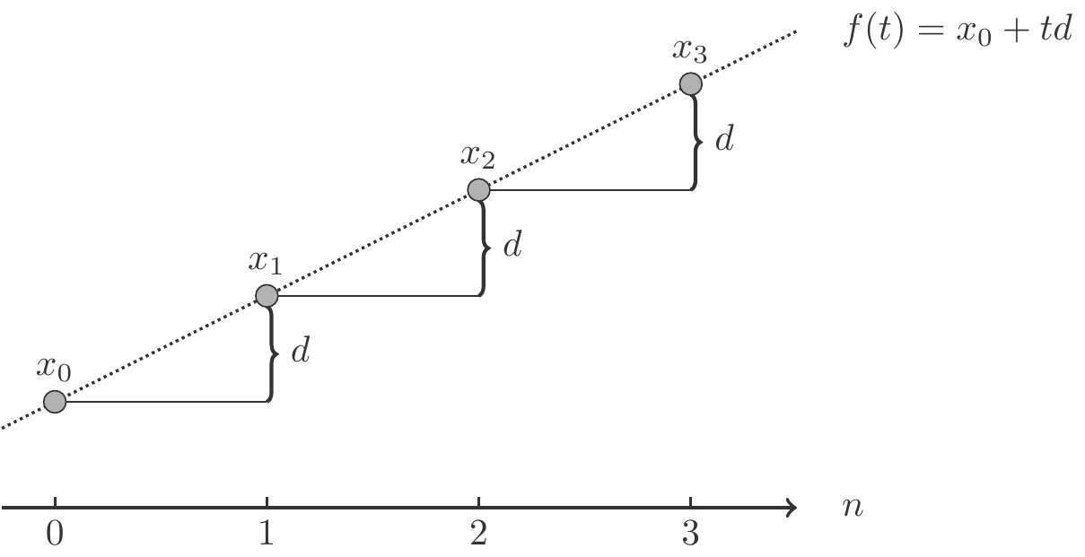
The qualitative course of the graph of an arithmetic sequence depends on the sign of the difference \(d\). We summarize the rather obvious facts in a theorem.
Theorem 1.24 Let \(x_n=x_0+nd\) be an arithmetic sequence.
(1) If \(d>0\), then the sequence \((x_n)\) is strictly increasing, i.e. \(x_n>x_{n-1}\) for all \(n=1,2,\ldots\).
(2) If \(d<0\), then the sequence \((x_n)\) is strictly decreasing, i.e. \(x_n<x_{n-1}\) for all \(n=1,2,\ldots\).
(3) If \(d=0\), then the sequence \((x_n)\) is constant, i.e. \(x_n=x_0\) for all \(n=1,2,\ldots\).
Applications
Let’s now consider a simple application of arithmetic sequences.
A company wants to produce 7,500 units of a product in the third year and reach a production level of 25,000 units after 10 years. The annual production increases should be constant. With how many units should production start in the first year, and how much should the annual increase be?
This problem can certainly be solved exclusively with common sense without any reference to arithmetic sequences. However, it is useful to make the mathematical structure of the problem clear even with such a simple task.
We denote the production figures of the individual years with \(x_1,x_2,\ldots, x_{10}\). If the production increases are to be constant annually, this means that the differences of this sequence are constant. Therefore, it is an arithmetic sequence. The sequence members \(x_3=7500\) and \(x_{10}=25\,000\) are specified. We need to calculate the member \(x_1\) and the difference \(\Delta x_n=d\).
Since now \(x_{10}-x_3=25000-7500=17500\) and moreover \[ \begin{gathered} x_{10}-x_{3}=(x_0+10d)-(x_0+3d)=7d,\end{gathered} \] it follows \(17\,500=7d\) and therefore \(d=2500\). The annual production increase must therefore be 2,500 units. To calculate the general sequence member, we compute the size of \(x_1\) from \[ \begin{gathered} x_3=x_0+3d=x_1+2d \quad \Rightarrow \quad x_1=x_3-2d=2500.\end{gathered} \] Therefore, our sequence is \[ \begin{gathered} x_n=x_0+nd=x_1+(n-1)d=2500+2500(n-1)=2500n,\end{gathered} \] and the starting value of production in the year \(n=1\) is \(x_1=2500\).
1.3.2 Summation of Sequences
Sum Formula
We now provide a formula that allows one to directly calculate the sum of an arithmetic sequence.
Theorem 1.26 The sum of the first \(n\) members of an arithmetic sequence \(x_1,x_2,\ldots,x_n\) amounts to \[ \begin{gathered} S_n=x_1+x_2+\cdots+x_n=n\cdot \dfrac{x_1+x_n}{2}.\end{gathered} \tag{1.8}\] This is \(n\) times the average value of the first and the last member of the sequence.
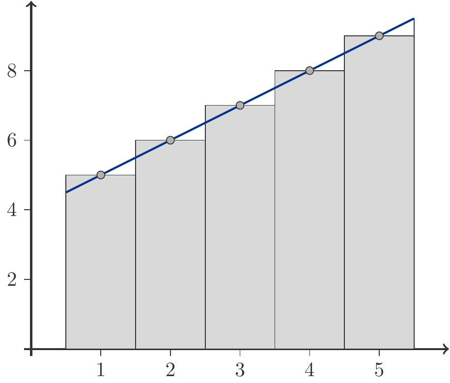
Remark 1.27 In Figure 1.8, the first five members of the arithmetic sequence \[ \begin{gathered} x_1=5,\;x_2=6,\;x_3=7,\;x_4=8,\;x_5=9\end{gathered} \] are illustrated by five bars, each of whose base is one and whose height corresponds to the respective sequence member.
The sum of the five sequence members is therefore identical to the sum of the areas of the five bars. This entire area is also identical to the area under the line that connects the five sequence members. When we calculate this area geometrically, we obtain exactly the formula (1.8): base length \(\times\) average height: \[ \begin{gathered} \frac{x_1+x_5}{2}\cdot 5=\frac{5+9}{2}\cdot 5=35.\end{gathered} \]
Now for the proof of the sum formula (1.8). The trick of proof is part of Western cultural history and therefore belongs to general education.
We write the sum twice, each time in the opposite order, and add up the overlying elements of the sequence: \[ \begin{gathered} \begin{array}{l@{\;=\;}l@{\;+\;}l@{\;+\cdots+\;}l} S_n & x_1 &x_2 &x_n\\ S_n &x_n&x_{n-1}&x_1\\ \hline 2S_n & (x_1+x_n) & (x_2+x_{n-1}) & (x_n+x_1) \end{array}\end{gathered} \tag{1.9}\] Now comes the punchline of the consideration: The sums \(x_1+x_n\), \(x_2+x_{n-1}\), …, \(x_n+x_1\) are all equal in size! Indeed, because \(x_2=x_1+d\) and \(x_n=x_{n-1}+d\), it follows, for example, that \[ \begin{gathered} x_2+x_{n-1}=(x_1+d)+x_{n-1}=x_1+(d+x_{n-1})=x_1+x_n. \end{gathered} \] Similarly, it can be shown that all other elements of the third line from (1.9) are also equal to \(x_1+x_n\). Therefore, the third line of (1.9) becomes \[ \begin{gathered} 2S_n=n(x_1+x_n),\end{gathered} \] which is already equivalent to our claimed formula. □
Remark 1.28 There are other ways to write the sum of \(n\) consecutive elements of an arithmetic sequence. If an arithmetic sequence starts with \(x_1\), then \(x_n=x_1+(n-1)d\). Thus \[ \begin{gathered} S_n=n\cdot\dfrac{x_1+x_n}{2}=\dfrac{n}{2}(2x_1+(n-1)d).\end{gathered} \]
Applications
Where do sums of arithmetic sequences occur in economic applications? Let’s start with a simple application example.
Exercise 1.29 A library lends books free of charge to students, with a maximum loan period of 14 days. If this time is exceeded, then the library charges a late fee of 6 GE per book for the first day, and this daily late fee increases by a further 2 GE per day. How much is the fine if one book is returned 8 days late?
Solution: The daily late fees form an arithmetic sequence with the initial value \(x_1=6\) and the difference \(d=2\), so \(x_n=6+2(n-1)\). Therefore, the late fee due for 8 days is: \[ \begin{gathered} S_8=\frac{8}{2}\left(x_1+x_8\right)=4(6+6+2\cdot 7)=104.\end{gathered} \] □
Exercise 1.30 The building land reserve of a small town currently amounts to 343,000 \(m^2\). While exactly 12,000 \(m^2\) will be built on in the current year, due to immigration and other factors, the newly built-up area increases by 2,400 \(m^2\) each year. After how many years will the town no longer have any building land reserves?
Solution: The area built on in the first year is \(x_1=12,000 \;m^2\), the area built on in the \(n\)-th year is \(x_n=12,000+2,400(n-1)\; m^2\). Thus, the consumption of building land over \(n\) years is: \[ \begin{gathered} \begin{array}{c@{\;=\;}l} S_n&x_1+x_2+\cdots+x_n=n\dfrac{24000+2400(n-1)}{2}\\[10pt] &12,000n+1,200n^2-1,200n=1,200n^2+10,800n\,. \end{array}\end{gathered} \] The building land reserve is used up when \(S_n\) reaches the value 343,000. Therefore, the quadratic equation has to be solved: \[ \begin{gathered} 1,200n^2+10,800n-343,000=0\,.\end{gathered} \] We solve this equation using the solution formula for quadratic equations: \[ \begin{gathered} ax^2+bx+c=0\implies x_{1,2}=\frac{-b\pm\sqrt{b^2-4ac}}{2a}.\end{gathered} \] This gives us two solutions: \[ \begin{aligned} &n_{1,2}=\frac{-10,800\pm\sqrt{10,800^2-4\cdot 1,200\cdot (-343,000)}}{2 \cdot 1,200} \\ &\implies\left\{\begin{array}{ccr} n_1 &=& 12.995\\ n_2&=&-21.995 \end{array}\right.\end{aligned} \] Only the positive solution \(n_1=12.995\approx 13\) is of interest to us. Hence, the building land reserves will be used up in just about 13 years. □
Arithmetically degressive depreciation is another application.
Exercise 1.31 An economic good with an acquisition value of 241,800 GE is to be written off arithmetically degressively over 12 years. That is, the depreciation amounts form a descending arithmetic sequence \(x_1,x_2,\ldots,x_{12}\) with \(x_{13}=0\). How should the depreciation amounts be chosen?
Solution: Complete depreciation within 12 years means that the sum of the depreciation amounts should equal the acquisition value. If the last depreciation amount is \(d\), then the sequence of depreciation amounts is as follows: \[ \begin{gathered} 12d,\,11d,\,10d,\ldots,\, 2d,\,d. \end{gathered} \] Therefore, it must be true: \[ \begin{aligned} 241,800 &=12d+11d+10d+\cdots+2d+d\\[5pt] &=12\cdot\frac{12d+d}{2}=78d.\end{aligned} \] Hence, \(d=3,100\). The first depreciation amount is \(x_1=12d=37,200\). It decreases annually by \(d=3,100\), i.e. \[ \begin{gathered} x_n=x_1-(n-1)d=37,200-(n-1)3,100,\end{gathered} \] until it finally ends at \(x_{12}=d=3,100\). □
The following problem comes from one of the most famous works of Leonhard Euler, Complete Introduction to Algebra. This book, widely distributed, appeared in 1770. On page 163 one finds:
Exercise 1.32 Someone buys a horse with the condition that they must pay 5 groats for the first horseshoe nail, 8 for the second, 11 for the third, and always 3 groats more for each subsequent one. However, there are 32 nails in total. How much must they pay for the horse?
Solution: Let \(x_n\) be the contribution of the \(n\)-th horseshoe nail to the purchase price. The \(x_n\) form an arithmetic sequence with \(x_1=5\) and \(d=3\), as well as \(x_n=5+3(n-1)\). The purchase price itself is calculated as the sum: \[ \begin{aligned} P&=x_1+x_2+\ldots+x_{32}=32\,\frac{x_1+x_{32}}{2}=16(5+5+31\cdot 3)\\[4pt] &= 1648 \text{ groats}.\end{aligned} \] Since in Euler’s times 30 groats were equal to one thaler, the purchase price was 54 thalers and 28 groats. □
1.4 Additional Exercises
-
In an operation, pipes are produced. The fixed costs for this production amount to 59400 CU (currency units), the variable costs are 157 CU per meter of pipe produced. When selling one meter of pipe, a revenue of 190 CU is earned. At how many meters of pipe is the break-even point reached?
Solution: \(1800\)
-
A hotel with 930 rooms makes a profit of 210 CU per day for each occupied room. An unoccupied room results in a loss of 100 CU per day. How many rooms must be occupied at the minimum to operate the hotel without loss?
Solution: \(300\)
-
The fixed costs for the acquisition of operating resources for the production of a good amount to 259578 CU. 69 units are produced per day, with production costs of 33 CU per unit. One unit is sold for 90 CU. After how many days of production does the company reach the break-even point?
Solution: \(66\)
-
A company anticipates production costs of 52 CU per unit for a new product. The fixed costs amount to 413480 CU. 440 units can be produced per month. At what price should the goods be sold if, after 11 months, a profit of 177000 CU is to be made?
Solution: \(174\)
-
A firm launches a new product on the market, with production costs of 70 CU per unit, and the calculated monthly fixed costs amount to 78000 CU. The company’s marketing department sets the price of the product such that the break-even point would be reached at a level of 2000 units. However, due to a design flaw detected too late, production has to be stopped after just 500 units. What is the loss incurred by the company due to this?
Solution: \(58500\)
-
An employment agency has 600 craftsmen under contract. If a craftsman can be placed as a temporary worker, the daily profit earned with this craftsman is 460 CU. However, a craftsman who is not employed results in a loss of 140 CU per day. How many of the craftsmen must be placed as temporary workers per day at a minimum for the agency to avoid losses?
Solution: \(140\)
-
A monopolist sells a good whose demand depends linearly on the set price. The monopolist achieves maximum revenue at a price of 100 CU. At this price, the demand is 20 units. What would the revenue be at a price of 160 CU?
Solution: \(1280\)
-
A company produces a good that it can sell at a legally fixed price of 138 CU. The fixed production costs amount to 176000 CU, and the variable costs in relation to the quantity produced \(q\) are \[ \begin{gathered} C_v(q)= 0.0053q^2+31q. \end{gathered} \] The company must pay a value-added tax of 19% of the sales revenue. What is the maximum profit the company can achieve if tax shifting to consumers is not possible due to legal measures?
Note: For a turnover of \(p\cdot q\) and a tax rate of \(t\), the amount of tax payable by the company is \(t\cdot p\cdot q\).
Solution: \(131802.28\)
-
A company can sell its product at a price of 100 CU (currency units). It produces with a cost function (\(x\) production quantity): \[ C(x)=x^2+6x+1480. \] At what sales quantity \(x_0\) does the company reach the break-even point?
Solution: \(20\)
-
A company produces with the cost function \(C(x)=24x+61200\). Currently, it has a monthly production capacity of 3600 units. What market price per unit must be achievable for the company to sell its maximum output without incurring a loss?
Solution: \(41\)
-
A company operates an underground parking garage in the city center with parking spaces exclusively for long-term parkers, with a minimum contract duration of 1 month. The garage can hold a maximum of 88 cars. An occupancy rate of 75% is achieved when the monthly fee per car is 600 CU. If the monthly fee were increased by 100 CU, it would result in the loss of a customer. What should be charged per parking space per month to maximize the operator’s revenue?
Solution: \(3600\)
-
A company produces a good that it can sell at a price of 90 CU. The fixed costs of production are 48200 CU, and the variable costs depending on the production quantity \(q\) are: \[ \begin{gathered} C_v(q)=\frac{1}{338} q^2+58q\,. \end{gathered} \] At which production quantity does the company achieve the highest profit?
Solution: \(5408\)
-
A monopolist has a demand function \(D(p)\) and a cost function \(C(q)\) given by \[ \begin{aligned} D(p): \;q &= -1.8665p+1230,\\ C(q) &= 0.4275q^2-168 q+79528 \end{aligned} \] At which production quantity \(q\) does it achieve maximum profit?
Solution: rounded \(429\)
-
An investment good valued at \(252,000\) CU should be depreciated using straight-line depreciation over \(5\) years. Calculate the first and the last depreciation amount.
Solution: \(x_1=84000, x_5=16800\).
-
Someone commits to paying a sum at the end of each year for 30 years, which increases by a constant amount year after year. The payment is 3900 CU in the 5th year and 5400 CU in the 20th year. How much needs to be paid in total over the 30 years, not considering any interest?
Solution: \(148500\)
-
14500 units of a product must be sold within 29 days. 150 units are sold on the first day. By how many units must the number of units sold daily be increased so that all goods are sold after 29 days?
Solution: \(25\)
-
In the first year the yield of a precious metal mine is 2500 tons per year, but this decreases evenly by 125 tons per year. At the current cost structure of the mining company, the break-even point is at 1625 tons. For how many more years can the mine be operated economically?
Solution: \(8\)
-
The financial authorities approve Company X AG to depreciate the newly acquired centrifugal casting machine using straight-line depreciation. Calculate the 9th depreciation amount when the cost of the machine is 376200 CU and it has a useful life of 11 years.
Solution: \(17100\)
-
In a parcel distribution center, 9700 packages must be allocated to individual delivery men within 25 hours. In the first hour, only 40 packages can be allocated. By how many units must the number of assigned packages per hour increase so that after 25 hours all packages are allocated?
Solution: \(29\)
The mineral oil tax is a prominent example of a quantity tax.↩︎