3 Differentiation
3.1 The Derivative of a Function
3.1.1 The Concept of Derivation
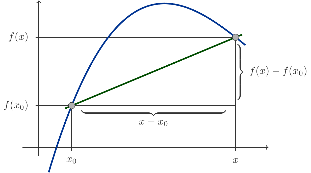
In our studies of linear functions in Section 1.1, we became acquainted with the rate of change of a function over an interval. The name rate of change points to a geometric property, and we are also familiar with the geometric interpretation of this property on the graph of the function. We now return to the concept of the rate of change in connection with non-linear functions.
Difference Quotient
Let \(f\) be a real function and \([x_0,x]\) an interval entirely contained within the domain of \(f\). The rate of change of the function \(f\) over the interval is calculated by the difference quotient \[ \begin{gathered} \frac{f(x)-f(x_0)}{x-x_0} \end{gathered} \tag{3.1}\] of the function on the interval \([x_0,x]\). This difference quotient is a very important quantity. We are reminded of its geometrical interpretation as the rate of change over the interval \([x_0,x]\). If one wants to interpret the difference quotient without reference to geometrical concepts, then it is viewed as the average change of the function over the interval \([x_0,x]\). The numerator of the formula (3.1) gives the total change \(f(x)-f(x_0)\) of the function on the interval, and when dividing this total change by the length \(x-x_0\) of the interval, we obtain the average change.

For linear functions, the difference quotient actually contains all the information one can obtain about how much the function changes. It does not matter which interval is used to calculate the difference quotient. For linear functions, every interval yields the same value because the rate of change is constant.
However, with non-linear functions, it’s different. Depending on which interval is used to calculate the difference quotient, a different value is obtained. This is not surprising, because the rate of change for non-linear functions is variable. To gain a complete overview, one would consequently need to specify the difference quotients (the rates of change) for all conceivable intervals on which the function is defined. However, this is very cumbersome and therefore, we are interested in how to gain an overview of the variable values of the rates of change for a non-linear function in a simpler manner.
The problem would become simpler if it were possible to define a measure which represents something like the rate of change of the function at a particular point. This is not entirely straightforward because there is no difference quotient at a point \(x_0\), namely \[ \begin{gathered} \frac{f(x_0)-f(x_0)}{x_0-x_0} \end{gathered} \tag{3.2}\] The quotient is nonsensical because both the numerator and the denominator equal zero. However, if we adopt the view that a very small interval around the point \(x_0\) would accomplish the same thing, then we are on the right track.
The Limit Transition
We consider a function \(y=f(x)\) and want to compute the slope ratio at the point \(x_0\). Since it is not possible, as already mentioned, to calculate a difference quotient at the point \(x_0\), we investigate small intervals that have the point \(x_0\) as an endpoint. Let \(x\) be a point close to \(x_0\), but different from \(x_0\). We want to know what values the difference quotient assumes as we move point \(x\) closer and closer to \(x_0\). Let’s look at an example.
Let \(f(x)=x^2\). We investigate the difference quotients for intervals that have \(x_0=2\) as one of their endpoints. The second endpoint of the intervals shall be \(x\). We choose \(x\) both to the right and to the left of \(x_0\) and approach \(x_0\) with \(x\) ever more closely. This approach is achieved by two sequences. The first sequence (left table) follows the rule \(x_n=2+1/(n+1)\), and the second sequence (right table) \(x_n=2-1/(n+1)\), each with \(n=1,2,3,\ldots\). Both sequences converge to the limit \(x_0=2\).
The resulting values of the difference quotient \(\frac{f(x_n)-f(x_0)}{x_n-x_0}\) are included in the following tables.
\[ \begin{gathered} \begin{array}{rcc} \hline n & x_n & \text{Difference Quotient}\\ \hline 1 & 2.500 & 4.500 \\ 2 & 2.250 & 4.250 \\ 3 & 2.125 & 4.125 \\ 4 & 2.063 & 4.063 \\ 5 & 2.031 & 4.031 \\ 6 & 2.016 & 4.016 \\ 7 & 2.008 & 4.008 \\ 8 & 2.004 & 4.004 \\ 9 & 2.002 & 4.002 \\ 10 & 2.001 & 4.001 \\ \hline \end{array}\qquad \begin{array}{rcc} \hline n & x_n & \text{Difference Quotient}\\ \hline 1 & 1.500 & 3.500 \\ 2 & 1.750 & 3.750 \\ 3 & 1.875 & 3.875 \\ 4 & 1.938 & 3.938 \\ 5 & 1.969 & 3.969 \\ 6 & 1.984 & 3.984 \\ 7 & 1.992 & 3.992 \\ 8 & 1.996 & 3.996 \\ 9 & 1.998 & 3.998 \\ 10 & 1.999 & 3.999 \\ \hline \end{array} \end{gathered} \]
From the tables, we can see that the values of the difference quotient apparently approach the number 4; they converge to 4! We have achieved this by using for the endpoints \(x\) of the intervals the start of a convergent sequence with the limit \(x_0=2\). Therefore, it is obvious to define the limit of the difference quotients as the value for the slope ratio of the function \(f(x)=x^2\) at the point \(x_0=2\).
Definition of the Derivative
The following definition now specifies what we mean by the slope ratio of a function at a point. The mathematical term for this concept is the derivative.
Definition 3.2 Let \(f\) be a function on an interval and \(x_0\) be an interior point of the interval.
If for every convergent sequence \(x_n, n=1,2,\ldots\) with \(x_n \ne x_0\), which approaches the limit \(x_0\), the sequence of difference quotients \[ \begin{gathered} \frac{f(x_n)-f(x_0)}{x_n-x_0} \end{gathered} \] is convergent and always towards the same limit, we call the function \(f\) differentiable at \(x_0\). The limit itself is called the derivative of the function \(f\) at \(x_0\) and is denoted by \(f'(x_0)\).
The notation often used is \[ \begin{gathered} f'(x_0):= \lim_{x \to x_0} \frac{f(x)-f(x_0)}{x-x_0}. \end{gathered} \tag{3.3}\] This indicates that a limit of the difference quotients exists for any sequence \(x_n \to x_0\), and this limit is called \(f'(x_0)\). Other notations and verbal forms are also commonly used. The process of calculating a derivative \(f'(x_0)\) is called differentiating the function. The derivative \(f'(x_0)\) is often referred to as the differential quotient and denoted by \[ \begin{gathered} f'(x_0)=\frac{df}{dx}(x_0). \end{gathered} \] This notation aims to suggest the resemblance of the derivative to a difference quotient. If one starts from a function equation \(y=f(x)\), it is even customary to write the derivative in the form \[ \begin{gathered} f'(x_0)=\frac{dy}{dx}(x_0) \end{gathered} \] although with this, the function \(f\) gets completely lost in the notation. Therefore, this designation should only be used when no misunderstandings can arise.
Derivative and Monotonicity
From the definition of the derivative, the following statements about the sign of the derivative are derived directly:
If the function \(f\) is monotonically increasing on the definition interval, then the derivative \(f'(x_0)\ge 0\).
If the function \(f\) is monotonically decreasing on the definition interval, then the derivative \(f'(x_0)\le 0\).
One can be even more precise about the relationship between the monotonicity of the function \(f\) and the sign of the derivative. This will be done in Section 3.4.1.
First Examples
Before we deal in detail with the intuitive interpretation of the derivative, let’s look at some concrete examples. In these examples, we compute derivatives through a limit process, as described in the definition of the derivative. However, this method of calculating derivatives is neither the simplest nor the usual approach. Instead, derivatives can be calculated much faster and easier using the rules of the so-called differential calculus. We will learn about these rules a bit later. The examples we are about to see now are only intended to better understand the definition of the derivative.
Let \(f(x)=ax+b\) be a linear function. Then, each difference quotient has the value \[ \begin{gathered} \frac{f(x)-f(x_0)}{x-x_0}=\frac{ax+b-ax_0-b}{x-x_0} =\frac{a(x-x_0)}{x-x_0}=a. \end{gathered} \] We have also seen this in Chapter 1. Therefore, as \(x\) approaches \(x_0\), the sequence of difference quotients is a constant sequence with the limit \[ \begin{gathered} \lim_{x\to x_0} \frac{f(x)-f(x_0)}{x-x_0}=\lim_{x\to x_0}a=a. \end{gathered} \] Thus, the derivative of a linear function is always \(f'(x_0)=a\), no matter at which point \(x_0\) the derivative is evaluated.
Let \(f(x)=2x^2+3x+1\) be a quadratic function. We calculate the derivative at a point \(x_0\) through a limit process using the difference quotient.
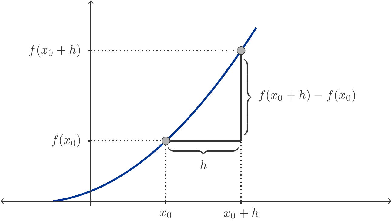
It is convenient and usually much clearer if we abbreviate the distance between the endpoints of the interval with a letter, for example, \(h:=x-x_0\). Then \(x=x_0+h\) and the limit \(x\to x_0\) is equivalent to \(h\to 0\) (compare Figure 3.2).
With this notation, the difference quotient is \[ \begin{aligned} \frac{f(x)-f(x_0)}{x-x_0}&= \frac{f(x_0+h)-f(x_0)}{h}\\ &= \frac{2(x_0+h)^2+3(x_0+h)+1-2x_0^2-3x_0-1}{h}\\ &= \frac{4x_0h+2h^2+3h}{h}\\ &= 4x_0+2h+3. \end{aligned} \] We now take the limit as \(h\to 0\) and obtain \[ \begin{aligned} f'(x_0) &= \lim_{h\to 0}\frac{f(x_0+h)-f(x_0)}{h} \\ &= \lim_{h\to 0} (4x_0+2h+3)=4x_0+3. \end{aligned} \] In this example, the derivative indeed depends on the point \(x_0\). For different points \(x_0\) we get different values of the derivative.
Let \(\displaystyle f(x)=\frac{1}{x}\). The difference quotient at a point \(x_0\not=0\) takes the form \[ \begin{aligned} \frac{f(x_0+h)-f(x_0)}{h} &= \frac{\dfrac{1}{x_0+h}-\dfrac{1}{x_0}}{h} \\ &= \frac{x_0-(x_0+h)}{h(x_0+h)x_0} \\ &= -\frac{1}{(x_0+h)x_0}. \end{aligned} \tag{3.4}\] By taking the limit as \(h\to 0\) we obtain \[ \begin{aligned} f'(x_0) &= \lim_{h\to 0}\frac{f(x_0+h)-f(x_0)}{h} \\ &= -\lim_{h\to 0} \frac{1}{(x_0+h)x_0}=-\frac{1}{x_0^2}. \end{aligned} \tag{3.5}\]
Let \(f(x)=\sqrt{x}\). The difference quotient at a point \(x_0>0\) is given by \[ \begin{gathered} \frac{f(x_0+h)-f(x_0)}{h}=\frac{\sqrt{x_0+h}-\sqrt{x_0}}{h}. \end{gathered} \] To determine the limit of the difference quotient for \(h\to 0\), we have to perform a clever transformation. We expand the fraction by multiplying numerator and denominator by \(\sqrt{x_0+h}+\sqrt{x_0}\) and use the well-known relationship \((a-b)(a+b)=a^2-b^2\): \[ \begin{gathered} \dfrac{\sqrt{x_0+h}-\sqrt{x_0}}{h}= \dfrac{(\sqrt{x_0+h}-\sqrt{x_0})(\sqrt{x_0+h}+\sqrt{x_0})}{h(\sqrt{x_0+h}+\sqrt{x_0})}\\ =\dfrac{x_0+h-x_0}{h(\sqrt{x_0+h}+\sqrt{x_0})}=\dfrac{1}{\sqrt{x_0+h}+\sqrt{x_0}}. \end{gathered} \] Now we can carry out the limit transition \(h\to 0\) and obtain \[ \begin{gathered} f'(x_0)=\dfrac{1}{2\sqrt{x_0}}. \end{gathered} \tag{3.6}\]
3.1.2 The Geometric Interpretation of the Derivative
We now turn to the interpretation of the concept of the derivative. Historically, the concept of the derivative has originated simultaneously from the solution to a geometric problem and from the solution to a dynamic problem. In this section, we will become familiar with the geometric interpretation.
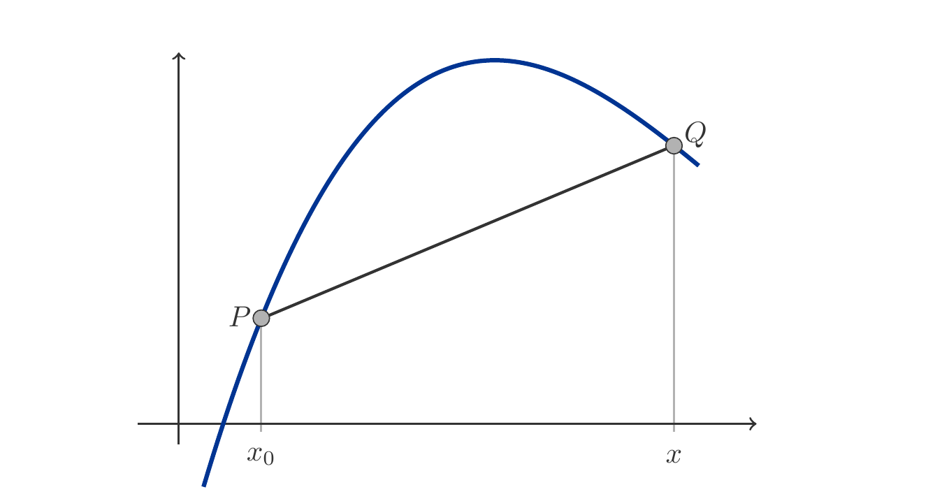
Let \(f\) be a function that is differentiable at point \(x_0\) and has the derivative \(f'(x_0)\). The geometric interpretation of the derivative is based on the geometric interpretation of the difference quotient. The difference quotient for the interval \([x_0,x]\) is the slope of the function on the interval \([x_0,x]\). If we connect the points \(P=(x_0,f(x_0))\) and \(Q=(x,f(x))\) with a straight line, a secant of the graph of the function is created, i.e., a line that intersects the graph of the function at two points (see Figure 3.3).
If we now let the \(x\)-coordinate of \(Q\) pass through a sequence of values \(x_1,x_2,x_3,\ldots\) that converge towards \(x_0\), then the secant changes. It becomes increasingly similar to the tangent at point \(P\), i.e., the line that touches the graph of the function at point \(P\). The process is illustrated in Figure 3.4.
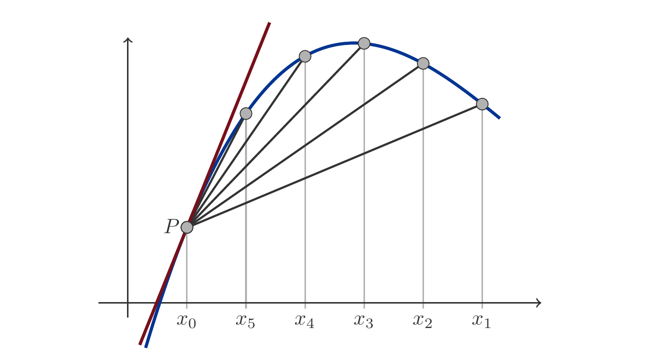
The tangent to the function graph at point \(P=(x_0,f(x_0))\) is a straight line that goes through point \(P\). Among the infinitely many straight lines that also pass through point \(P\), the tangent is the only one whose slope ratio matches the derivative \(f'(x_0)\) of the function \(f\) at point \(x_0\). Hence, the equation of the tangent is1 \[ \begin{gathered} y=f'(x_0)(x-x_0)+f(x_0). \end{gathered} \tag{3.7}\] Thus, we can express the geometric interpretation of the derivative as:
Theorem 3.7 The derivative of a differentiable function at a point \(x_0\) is equal to the slope of the tangent to the graph of the function at the point \(x_0\).
Existence of the Derivative
The examples and geometric considerations just discussed may have created the impression in readers that functions that possess a derivative are not really anything special. But that is not the case at all. On the contrary, in Definition 3.2, two very strict conditions are formulated. The sequence of difference quotients must converge for every sequence \(x_n\) approaching \(x_0\), and it must always converge to the same limit. This is by no means self-evident.
A necessary condition for the existence of the derivative of a function is its continuity. Continuity is a fundamental concept in modern mathematics, and it is a difficult concept. Therefore, we want to leave it at that and develop an intuitive understanding of it here. For this, we refer to Leonhard Euler, who wrote in 1748:
A function is continuous on an interval if its graph can be drawn with a pencil in that interval without lifting the pencil from the paper.
Euler meant that the graph of the function must not have any breaks or holes, that small changes in the variable \(x\) only cause small changes in the function value \(f(x)\). The function \(f(x)\) in Figure 3.5 is discontinuous at the point \(x=0\). It has a jump discontinuity there.

Functions like the one shown in Figure 3.5 are by no means pathological exceptions. In Chapter 5, we will encounter distribution functions of discrete random variables that exhibit exactly this kind of behavior.
But continuity alone is not sufficient. For a function to be differentiable at all points of an interval, it must be not only continuous there but also smooth. What does the attribute smooth mean in this context? It means that a function, for example, must not have any corners.
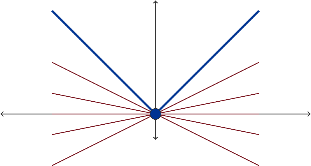
The seemingly harmless function \(f(x)=|x|\) is not so innocuous after all. Its graph in Figure 3.6 fits into Euler’s vision of continuity. But at \(x_0=0\), \(f(x)\) has a corner. And it is quite obvious: The position of the tangent cannot be determined unambiguously at this point. In fact, any linear function \(y=kx\) is a tangent at \(x_0=0\), as long as \(-1\le k\le 1\).
3.2 Differentiating
Let \(y=f(x)\) be a function that is differentiable on an interval \((a,b)\). To calculate the derivative \(f'(x)\) for every point \(x\in(a,b)\), we would have to form the limit of the difference quotient for each \(x\). But often it can be simpler. There are straightforward rules for calculating the derivative of an elementary function as a formula without having to form a limit. These so-called rules for differentiating can be mechanically applied (calculus) and can therefore also be entrusted to machines.
In this section, we will learn the rules for differentiating, and we also want to be able to apply them to simple tasks. It is not the essence of calculus to be able to differentiate complex function terms by hand without error. We can confidently leave that to computer programs. But we do want to understand the principles upon which differentiation is based.
Most function terms encountered in differentiation consist of very simple components that are linked by operations such as addition and multiplication. Furthermore, function terms are created through composition, the formation of inverse functions, and the formation of powers. If we understand how to deal with these operations in differentiation, then we are prepared for many situations.
3.2.1 Basic Differentiation Rules
Let’s start with rules that we already know. The derivative of a linear function \(f(x)=ax+b\) is \(f'(x)=a\) for all \(x\in\mathbb R\). The derivative is simply the slope ratio, which for a linear function is constant. The exact proof was provided in Example 3.3. For what comes next, two special cases are important:
Theorem 3.8 The derivative of a constant function \(f(x)=b\) is \(f'(x)=0\) for all \(x\in\mathbb R\).
The derivative of the function \(f(x)=x\) is \(f'(x)=1\) for all \(x\in\mathbb R\).
At first, we are interested in all those functions that we can obtain from linear functions through multiplication and addition. For this purpose, we consider in general how adding and multiplying function terms affect the formation of derivatives. The sum rule and the product rule answer these questions.
Theorem 3.9 (Sum Rule) If \(y=f(x)\) and \(y=g(x)\) are differentiable functions, then their sum \(f(x)+g(x)\) is also a differentiable function and it holds \[ \begin{gathered} (f(x)+g(x))'=f'(x)+g'(x). \end{gathered} \tag{3.8}\]
One can justify the sum rule by providing a precise formal proof in which one examines the difference quotients and carries out the transition to the derivative according to Definition 3.2. However, we refrain from this kind of strict proof. Instead, we try to understand the sum rule intuitively, and this is just as important as the formal proof. An intuitive understanding is reached through a heuristic consideration2.
To understand the sum rule, we recall that with small changes from \(x\) to \(x+h\), we can approximate the change in function values by the derivative (calculate approximately): \[ \begin{gathered} \begin{array}{lcl} f(x+h)-f(x) &\approx& f'(x)h, \\ g(x+h)-g(x) &\approx& g'(x)h. \end{array} \end{gathered} \tag{3.9}\] This local linearization is the key to any intuitive handling of the concepts of differential calculus. If we then calculate the change in the sum function \(f+g\), the addition of the two equations in (3.9) results in: \[ \begin{aligned} & \left[f(x+h) + g(x+h)\right] - \left[f(x)+g(x) \right] \\ = & \left[f(x+h)-f(x) \right] + \left[g(x+h)-g(x) \right]\\ \approx & \left[f'(x)+g'(x) \right]h. \end{aligned} \] We see: Because the change of a sum is equal to the sum of the changes of the terms, it is plausible that the derivative of a sum is equal to the sum of the derivatives.
Let’s look at a simple, but important special case.
Let \(y=f(x)\) be a differentiable function and let \(c\in\mathbb R\) be a number. What is the derivative of \(h(x)=f(x)+c\)?
The answer is easily found using the sum rule. The function \(h\) is a sum of two differentiable functions. Therefore, it holds \[ \begin{gathered} h'(x)=(f(x)+c)'=f'(x)+(c)'=f'(x)+0=f'(x). \end{gathered} \] This makes it clear: An additive constant disappears when differentiating.
The product rule is a bit more complicated than the sum rule. We start with a heuristic consideration to understand what is actually happening.
Let \(A,\,a,\,B,\,b\) be any numbers. We are familiar with the fact that \[ \begin{gathered} (A+a)(B+b)=AB+aB+Ab+ab. \end{gathered} \tag{3.10}\] Now, let’s imagine that \(A\) and \(B\) are two numbers that are very large compared to \(a\) and \(b\). For example, \(A=1000\), \(B=3000\), \(a=15\) and \(b=20\). We are interested in the difference of the products \((A+a)(B+b)\) and \(AB\). For our numerical example, we can simply calculate the difference: \[ \begin{gathered} (A+a)(B+b)-AB=3065300-3000000=65300. \end{gathered} \] However, if we want to know in general what components this difference consists of, we must apply (3.10) and get \[ \begin{gathered} (A+a)(B+b)-AB=aB+Ab+ab, \end{gathered} \] and in our numerical example \[ \begin{gathered} 65300=45000+20000+300. \end{gathered} \] From this, we see that the third term \(ab\) contributes little. The determining components are \(aB\) and \(Ab\), so \[ \begin{gathered} (A+a)(B+b)-AB\approx aB+Ab. \end{gathered} \] The Figure 3.7 shows this fact very clearly.
We will see that the product rule for differentiation follows exactly this formula: change in the first factor times the value of the second factor plus the value of the first factor times the change of the second factor.
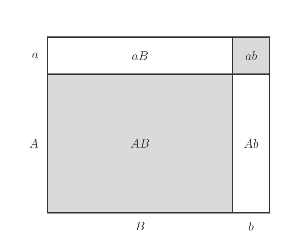
We again assume that we are dealing with functions for which the equations (3.9) apply, but which we now slightly modify in the form \[ \begin{gathered} \begin{array}{lcl} f(x+h) &\approx& f(x)+f'(x)h, \\ g(x+h) &\approx& g(x)+g'(x)h. \end{array} \end{gathered} \] If we now calculate the change of the product function \(fg\), we obtain \[ \begin{aligned} & f(x+h)g(x+h) \\ \approx & [f(x)+f'(x)h][g(x)+g'(x)h]\\ = & f(x)g(x)+f'(x)g(x)h+f(x)g'(x)h+f'(x)g'(x)h^2. \end{aligned} \] The geometric interpretation of this development of a product into four summands is hinted at in the Figure 3.7. Since we always deal with small changes \(h\), \(h^2\) is especially small, and therefore the fourth summand is negligible. We, therefore, finally obtain \[ \begin{gathered} f(x+h)g(x+h)-f(x)g(x)\approx [f'(x)g(x)+f(x)g'(x)]h \end{gathered} \] This leads us to suspect that the derivative of the product \(f(x)g(x)\) must be equal to \(f'(x)g(x)+f(x)g'(x)\).
Theorem 3.12 (Product Rule) If \(y=f(x)\) and \(y=g(x)\) are differentiable functions, then their product \(f(x)\cdot g(x)\) is also a differentiable function and it holds that \[ \begin{gathered} \ [f(x)g(x)]'=f'(x)g(x)+f(x)g'(x). \end{gathered} \tag{3.11}\]
We now turn to a very simple but important special case.
Let \(y=f(x)\) be a differentiable function and let \(c\in\mathbb R\) be a number. What is the derivative of \(h(x)=cf(x)\)?
The answer is found easily with the product rule. The function \(h(x)\) is a product of two differentiable functions. Therefore, we have \[ \begin{gathered} \begin{array}{rcrcll} h'(x)=[cf(x)]' & = & (c)' f(x) & + & cf'(x) & \\ & = & 0\;\;f(x) & + & cf'((x) & = cf'(x). \end{array} \end{gathered} \] This makes it clear: A constant factor remains unchanged when differentiating.
These two rules, the sum rule and the product rule, suffice to differentiate a large number of functions, especially all polynomials successfully.
The next example is actually no longer a special case of the product rule, but an independent rule for differentiating power functions with positive integer exponents.
We want to differentiate \(f(x)=x^n\) with natural exponents \(n\in\mathbb N\) . We already know a special case of this. For \(n=1\), \(f(x)=x\) and we have \(f'(x)=1\).
Let us now consider the function \(f(x)=x^2\). The difference quotient reads \[ \begin{gathered} \frac{f(x+h)-f(x)}{h}=\frac{(x+h)^2-x^2}{h}=2x+h. \end{gathered} \] After taking the limit \(h\to 0\), we get \(f'(x)=2x\).
We now claim that the general rule for the derivative of power functions is \[ \begin{gathered} f(x)=x^n \quad\Rightarrow\quad f'(x)=nx^{n-1}. \end{gathered} \tag{3.12}\] As we have seen, this rule is certainly correct for the cases \(n=1\) and \(n=2\). We now prove it for the case \(n=3\). For this, we use the product rule: \[ \begin{gathered} (x^3)'=(x^2\cdot x)'=(x^2)'x+x^2(x)'=2x\cdot x+x^2\cdot 1=3x^2. \end{gathered} \] So our rule is also correct for \(n=3\). One can now continue in this way to prove the rule for all \(n\in\mathbb N\). If we have proven it for \(n=k-1\), then it automatically follows from the product rule \[ \begin{aligned} (x^k)' = (x^{k-1}\cdot x)' & = (x^{k-1})'x+x^{k-1}(x)' \\ & = (k-1)x^{k-2}\cdot x+x^{k-1}\cdot 1=kx^{k-1}. \end{aligned} \] Thus the rule is also correct for \(n=k\).
Now we are able to differentiate any polynomial: \[ \begin{gathered} \begin{array}{ll} f(x)=a & f'(x)=0\\ f(x)=ax+b & f'(x)=a\\ f(x)=ax^2+bx+c &f'(x)=2ax+b\\ \ldots \end{array} \end{gathered} \]
When a function term can be represented as a product of two functions, it is usually easier to apply the product rule directly rather than expanding (developing) the function term.
Exercise 3.15 The derivative of the function \(h(x)=x^4(5x^2-1)\) is sought.
Solution: We set \(f(x)=x^4\) and \(g(x)=5x^2-1\). Then we get \[ \begin{aligned} h'(x) & =f'(x)g(x)+f(x)g'(x) \\ & =4x^3(5x^2-1)+x^4\cdot 10x=30x^5-4x^3. \end{aligned} \] □
We conclude our applications of the product rule with an example, the solution of which we already know.
We know from Example 3.5 that the function \(f(x)=1/x\) is differentiable for \(x\not=0\) and what the derivative looks like. However, it is interesting to see how the derivative can also be found using the product rule.
After all, \(xf(x)=1\) and if we differentiate both sides of the equation, we must obtain identical derivatives. Therefore, we have \[ \begin{gathered} (xf(x))'=(1)'=0, \end{gathered} \] and therefore \[ \begin{gathered} 1f(x)+xf'(x)=0. \end{gathered} \] From this equation we can calculate \(f'(x)\) and get \[ \begin{gathered} f'(x)=-\frac{f(x)}{x}=-\frac{1}{x^2}. \end{gathered} \tag{3.13}\]
3.2.2 The Chain Rule
Addition and multiplication are not the only operations for forming new function terms from given ones. The composition of terms plays just as big a role.
To compose means to insert one function into another. So if we have two functions \(z=f(y)\) and \(y=g(x)\), then we can form the composition \(f(g(x))\) by replacing \(y\) in \(f(y)\) with \(g(x)\). The function \(f(y)\) into which the substitution is made, we call the outer function, the function that is substituted is called the inner function.
If, for example, \(f(y)=\sqrt{y}\) and \(g(x)=1+x^2\), then we have \[ \begin{gathered} f(g(x))=\sqrt{g(x)}=\sqrt{1+x^2}. \end{gathered} \] Note that composition is not commutative. In our example, we get: \[ \begin{gathered} g(f(y))=1+(f(y))^2=1+(\sqrt{y})^2 =1+y. \end{gathered} \]
The following chain rule is precisely intended for differentiating such compositions. It is certainly the most important and consequential rule for forming derivatives.
Before we formally state the chain rule as a theorem, let’s try to get a heuristic grip on the problem again. Let’s start with an example.
Let \(f(y)=ay+b\) and \(g(x)=cx+d\) be two linear functions. It is clear that \(f'(y)=a\) and \(g'(x)=c\). We compose the two functions and thus obtain \[ \begin{gathered} f(g(x))=f(cx+d)=a(cx+d)+b=acx+ad+b. \end{gathered} \] The result of the composition is a linear function with the slope ratio \(ac\), thus \([f(g(x)]'=ac\). We therefore notice that in the case of linear functions \[ \begin{gathered} \ [f(g(x))]'=f'(y)g'(x) \end{gathered} \] holds. It will turn out that this formula is generally correct for nonlinear functions as well.
Let \(z=f(y)\) and \(y=g(x)\) be two differentiable functions that can be composed to \(f(g(x))\). We again assume that for small changes \(h\) and \(k\), linear approximations using the derivatives \[ \begin{gathered} \begin{array}{lcl} f(y+h) &\approx& f(y)+f'(y)h,\\ g(x+k) &\approx& g(x)+g'(x)k \end{array} \end{gathered} \] are possible. If we now examine the composed function \(f(g(x))\) at the point \(x+k\), we see that \[ \begin{gathered} f(g(x+k))\approx f(g(x)+g'(x)k). \end{gathered} \] Now \(g(x)\) takes on the role of \(y\) and \(g'(x)k\) the role of \(h\). This leads to \[ \begin{gathered} \begin{array}{lcl} f(g(x+k))&\approx& f(g(x)+g'(x)k)\\ &=& f(y+h)\approx f(y)+f'(y)h\\ &=& f(g(x))+f'(g(x))g'(x)k. \end{array} \end{gathered} \] This simply means that \[ \begin{gathered} f(g(x+k))- f(g(x))\approx f'(g(x))g'(x)\cdot k. \end{gathered} \] Therefore, the candidate for the derivative of \(f(g(x))\) is the product of the outer derivative \(f'\) and the inner derivative \(g'\).
Theorem 3.18 (Chain Rule) Let \(z=f(y)\) and \(y=g(x)\) be two differentiable functions that can be composed to \(f(g(x))\). Then the composed function is also differentiable and the following holds \[ \begin{gathered} \ [f(g(x))]'=f'(g(x))\cdot g'(x). \end{gathered} \tag{3.14}\] The chain rule has a very simple structure. It states the following:
The derivative of a pair of composed functions is equal to the product of the derivatives of the individual functions.
Exercise 3.19 Differentiate the function \(h(x)=(1+x^2)^{10}\).
Solution: Let \(f(y)=y^{10}\) and \(y=g(x)=1+x^2\). Then \(h(x)=f(g(x))=g^{10}(x)\) and we get \[ \begin{gathered} h'(x)=f'(g(x))g'(x)=10g^{9}(x)\cdot 2x= 20x(1+x^2)^{9}. \end{gathered} \] □
Let \(g\not=0\) be a differentiable function. We want to differentiate the function \[ \begin{gathered} h(x)=\frac{1}{g(x)} \end{gathered} \] For this, we can use the chain rule. Letting \(y=g(x)\) and \(\displaystyle f(y)=1/y\), so that \(h(x)=f(g(x))\), it follows from (3.13) \[ \begin{gathered} h'(x)=f'(g(x))g'(x)=-\frac{g'(x)}{g^2(x)}. \end{gathered} \tag{3.15}\]
We want to find the derivative of \(\displaystyle f(x)=1/x^n\) for \(n\in\mathbb N\). Using (3.15) we discover \[ \begin{gathered} f'(x)=-\frac{nx^{n-1}}{x^{2n}}=-\frac{n}{x^{n+1}}=-nx^{-n-1}. \end{gathered} \]
The quotient rule describes how to find the derivative of a quotient \(f(x)/g(x)\) from the derivatives of the numerator and denominator. It holds that \[ \begin{gathered} \left( \frac{f(x)}{g(x)} \right)'=\frac{f'(x)g(x)-f(x)g'(x)}{g^2(x)}. \end{gathered} \tag{3.16}\] This rule emerges from the product rule and from (3.15). It results in \[ \begin{gathered} \left( \frac{f}{g} \right)'=\left( f\frac{1}{g} \right)'= f'\frac{1}{g}+f\left(\frac{1}{g}\right)' =\frac{f'}{g}-f\frac{g'}{g^2}=\frac{f'g-fg'}{g^2}. \end{gathered} \]
Exercise 3.23 Differentiate the function \(\displaystyle h(x)=(3x-2)/(x+1)\) using the quotient rule.
Solution: We have \(f(x)=3x-2\) and \(g(x)=x+1\). \[ \begin{gathered} h'(x)=\frac{3(x+1)-(3x-2)\cdot 1}{(x+1)^2}=\frac{5}{(x+1)^2}. \end{gathered} \] □
With the chain rule, we can also differentiate inverse functions if we know the derivative of the original function.
Let \(y=f(x)\) and \(x=g(y)\) be continuous functions that are inverses of each other. Examples of such pairs of inverse functions have been known to us for a long time, for example: \[ \begin{gathered} y=x^2,\quad x=\sqrt{y},\\ y=e^x,\quad x=\ln y. \end{gathered} \] We assume that \(f\) is a differentiable function. Before we can calculate a derivative of the inverse function, we need to consider whether the inverse function is differentiable at all.
We will do this in a pictorial heuristic way. The differentiability of the inverse function \(g\) can only fail if there are angular points or vertical tangents. However, angular points cannot occur because the graphs of \(f\) and \(g\) are identical, and the graph of \(f\) has no angular points. A vertical (i.e., parallel to the \(x\)-axis!) tangent occurs in the graph of \(x=g(y)\) where the graph of \(y=f(x)\) has a horizontal tangent, that is, where \(f'(x)=0\). Such points must therefore be excluded.
Thus, \(g\) is differentiable at all points \(y=f(x)\) where \(f'(x)\not=0\). From \(f(g(y))=y\), by forming the derivative on both sides, we get \[ \begin{gathered} f'(g(y))g'(y)=1, \end{gathered} \] and therefore \[ \begin{gathered} g'(y)=\frac{1}{f'(g(y))}=\frac{1}{f'(x)},\quad \text{where $x=g(y)$ and $y=f(x)$.} \end{gathered} \tag{3.17}\] We see: The derivative of the inverse function is the reciprocal of the derivative of the original function.
We are familiar with the derivative of \(g(x)=\sqrt{x}\) from Example 3.6. However, we can reach the same result by a different approach.
The function \(g\) is the inverse function of \(x=f(y)=y^2\) with the derivative \(f'(y)=2y\). From this we have \[ \begin{gathered} g'(x)=\frac{1}{f'(g(x))}=\frac{1}{2g(x)}=\frac{1}{2\sqrt{x}}. \end{gathered} \]
3.2.3 Exponential Function and Logarithm
Finally, we need to deal with the derivative of exponential functions and logarithmic functions. The fundamental theorem from which everything else follows intuitively is the rule for deriving the exponential function \(f(x)=\exp(x)=e^x\).
Theorem 3.26 The exponential function \(f(x)=\exp(x)=e^x\) is differentiable and it holds \[ \begin{gathered} f'(x)=\exp(x)=e^x. \end{gathered} \tag{3.18}\]
Thus, the exponential function \(\exp(x)=e^x\) reproduces itself when differentiated. This property is remarkable. In fact, it can be demonstrated that no other function has this characteristic. However, what interests us most is understanding why the exponential function has this beautiful property. And grasping this heuristically is not at all difficult. Remember that \[ \begin{gathered} e^x=\lim_{n\to\infty} \Big(1+\frac{x}{n}\Big)^n. \end{gathered} \tag{3.19}\] It is therefore plausible to suspect that the properties of \(e^x\) can be explained by the properties of the sequence of functions \[ \begin{gathered} g_n(x)=\Big(1+\frac{x}{n}\Big)^n \end{gathered} \] When we differentiate the functions \(g_n(x)\), we get (using the chain rule) \[ \begin{gathered} g_n'(x)=n\Big(1+\frac{x}{n}\Big)^{n-1}\frac{1}{n}= \Big(1+\frac{x}{n}\Big)^{n-1}=\frac{g_n(x)}{1+\dfrac{x}{n}}\,. \end{gathered} \] Thus, \(g_n(x)\) almost reproduces itself upon differentiation, and the deviation from exact replication decreases as \(n\) increases. Together with (3.19), although this is not a strict proof of Theorem 3.26, it is a clue that the statement of Theorem 3.26 is not entirely incomprehensible.
In most applications, however, we encounter the exponential function in composite form, that is, we are dealing with functions of the form \(y=e^{f(x)}\). Their derivative must obviously be formed using the chain rule. The outer derivative is then obtained from Theorem 3.26:
Theorem 3.27 Let \(g(x)=e^{f(x)}=e^y\) with \(y=f(x)\). Then: \[ \begin{gathered} g'(x)=e^y\cdot y'=e^{f(x)}\cdot f'(x)\,. \end{gathered} \tag{3.20}\]
Exercise 3.28 Differentiate \(f(x)=3e^{-5x^2}\).
Solution: To find the derivative of \(f\), we apply the chain rule (3.20): \[ \begin{gathered} f'(x)=3e^{-5x^2}(-10x)=-30xe^{-5x^2}. \end{gathered} \] □
Now, the general case.
Let \(f(x)=a^x\) be an exponential function with an arbitrary positive base. From (2.37), we know that such an exponential function can be written in the form \[ \begin{gathered} f(x)=a^x=e^{x\ln a} \end{gathered} \tag{3.21}\] In this form, it is not difficult to compute the derivative. Applying the chain rule we get \[ \begin{gathered} f'(x)=e^{x\ln a}\ln a=a^x\ln a. \end{gathered} \tag{3.22}\]
Exercise 3.30 Find the first derivative of the function \(y=3^{x^2+1}\).
Solution: We start by expressing \(y\) as Euler’s exponential function, so that we can apply (3.20): \[ \begin{gathered} y=3^{x^2+1}=e^{(x^2+1)\ln 3} \end{gathered} \] Using the chain rule we obtain: \[ \begin{gathered} y'=e^{(x^2+1)\ln 3}\cdot 2x\cdot\ln 3=2x\ln 3\cdot 3^{x^2+1} \end{gathered} \] □
The derivative of the logarithm function \(g(x)=\ln x\) can be derived by the chain rule.
Let \(g(x)=\ln x\). Then \(e^{g(x)}=x\) and by taking the derivative on both sides we get: \[ \begin{gathered} e^{g(x)}g'(x)=1. \end{gathered} \] From this, \[ \begin{gathered} g'(x)=\frac{1}{e^{g(x)}}=\frac{1}{e^{\ln x}}=\frac{1}{x}. \end{gathered} \tag{3.23}\]
Like the exponential function, the logarithmic function in most applications is encountered in a composed form. The chain rule, combined with (3.23), solves the problem.
Theorem 3.32 (Logarithmic derivative) Let \(g(x)=\ln f(x)=\ln y\) where \(y=f(x)\). Then: \[ \begin{gathered} g'(x)=\left(\ln f(x)\right)'=\frac{f'(x)}{f(x)}. \end{gathered} \tag{3.24}\]
Exercise 3.33 We are looking for the first derivative of \(y=\ln(3x^2-4x+1)\).
Solution: This \(y\) is exactly of the form \(\ln f(x)\) with \(f(x)=3x^2-4x+1\). Using (3.24) we find: \[ \begin{gathered} y'=\frac{6x-4}{3x^2-4x+1}. \end{gathered} \] □
The last differentiation rule we need is for general power functions \(f(x)=x^{\alpha}\). So far, we can only find the derivative \(f'(x)\) for integer \(\alpha\), see (3.12).
The general rule looks just like the case of integer exponents.
Theorem 3.34 (Derivative of power functions) Let \(f(x)=x^\alpha\) with \(\alpha\in\mathbb R\). Then: \[ \begin{gathered} f'(x)=\alpha x^{\alpha-1}. \end{gathered} \tag{3.25}\]
Justification: This is easy to see if we write \(x^\alpha\) as an exponential function. After all, \(f(x)=x^\alpha=e^{\alpha\ln x}.\) From this, the chain rule implies \[ \begin{gathered} f'(x)=e^{\alpha\ln x}\,\alpha\,\frac{1}{x}=x^\alpha\,\alpha\,\frac{1}{x}= \alpha x^{\alpha-1}. \end{gathered} \] □
We conclude this section with one final example:
Exercise 3.35 We are looking for the first derivative of the function \(y=x^x\).
Solution: Again, we begin by expressing \(y\) as the Eulerian exponential function: \[
\begin{gathered}
y=x^x = e^{x\ln x}.
\end{gathered}
\] Utilizing
(3.20) and the product rule for the inner derivative yields: \[
\begin{aligned}
y'&=e^{x\ln x}\left(x\ln x\right)'= e^{x\ln x}\left(1\cdot\ln
x+x\cdot\frac{1}{x}\right)\\[4pt]
&=x^x\left(\ln x +1\right).
\end{aligned}
\] □
3.3 Interpretations of the Derivative
3.3.1 Velocity
The dynamic interpretation of the derivative is associated with the concept of velocity. Let \(y=f(t)\) be a function that indicates a state of an object or system. Here, \(t\) denotes the time at which the state is measured.
Change in Position
A vehicle moves along a road. It starts at time \(t_0\) from a specific point, marked with the kilometer marker \(f(t_0)\). For every moment \(t>t_0\), \(f(t)\) is the kilometer marker of the point on the road where the vehicle is at that time.
When the time duration \(t-t_0\) has passed, the vehicle has covered the distance \(f(t)-f(t_0)\). The difference quotient \[ \begin{gathered} \frac{f(t)-f(t_0)}{t-t_0} \end{gathered} \] indicates how large the distance was that the vehicle averagely covered per unit of time. This difference quotient is called the average velocity of the vehicle over the time interval \([t_0,t]\).
One says that the vehicle moves uniformly if the covered path \(f(t)\) is a linear function, meaning \(f(t)=vt+b\). In this case, for every time interval, the difference quotient and thus the average velocity equal \(v\). It is then justified to call \(v\) the velocity of the vehicle.
If the vehicle does not move uniformly, then the covered path \(f(t)\) is some nonlinear function. The average velocity can then differ across various intervals. How should one define the velocity of the vehicle at a particular moment in such a situation?
The answer to this question is the concept of instantaneous velocity. We assume that the function \(y=f(t)\) is differentiable. Then we calculate the average velocities for smaller and smaller intervals \([t_0,t]\). The limit of these average velocities is the derivative \[ \begin{gathered} f'(t_0)=\lim_{t\to t_0} \frac{f(t)-f(t_0)}{t-t_0} \end{gathered} \] of the function \(f\) at the point \(t_0\). This limit is called the instantaneous velocity of the vehicle at the moment \(t_0\). The instantaneous velocity is therefore the derivative of the function that indicates the covered path.
3.3.2 Rates of Change
Let’s return to the general situation. The difference quotient \[ \begin{gathered} \frac{f(t)-f(t_0)}{t-t_0} \end{gathered} \tag{3.26}\] indicates the average change of the state in the time interval \([t_0,t]\). Such a metric, which relates the change to the time it requires, is generally called a rate of change or simply a rate. From this perspective velocity of a vehicle is the rate of change in position. The instantaneous rate of change is then the derivative of the state function \(f\), meaning \[ \begin{gathered} f'(t_0)=\lim_{t\to t_0}\frac{f(t)-f(t_0)}{t-t_0}. \end{gathered} \tag{3.27}\] In summary:
Theorem 3.36 The derivative of a differentiable function \(f(t)\) at a point \(t_0\) is the instantaneous rate of change of the function at the point \(t_0\).
Exercise 3.37 Between \(1990\) and \(2010\), a company significantly increased its turnover. A statistical analysis of the annual turnovers revealed that they can be well approximated by the function \[ \begin{gathered} f(t)= 5+0.1t+0.01t^2 \quad\text{in million CU},\quad 1990: t=0. \end{gathered} \]
What was the average turnover growth between \(1995\) and \(2000\)?
What was the (instantaneous) growth rate in \(1998\)?
Before we get to answering these questions, a word about the given function \(f(t)=5+0.1t+0.01t^2\). It is an example of a quadratic trend function. When we plot yearly sales in a 2-dimensional coordinate system, we get the image of a scatter plot \((t_i, f(t_i))\), where \(t_i\) is the year \(i\), \(f(t_i)\) the sales of the year \(t_i\). Now, using methods that statistics and econometrics provide, a trend function can be fitted through this scatter plot, which approximates the points as well as possible, see Figure 3.8 for illustration.
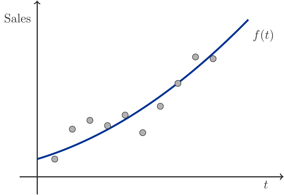
The purpose of these trend functions is on the one hand to have simple explanatory models (for example for the sales development), on the other hand, they can also be used for forecasts.
Solution:
(a) We investigate the function \(f(t) = 5 +0.1\;t + 0.01\;t^{2}\). The average growth over the interval \([t_{0},t]\) is given by the difference quotient \[ \begin{gathered} \dfrac{f(t)-f(t_{0})}{t-t_0} \end{gathered} \] First, we determine: \[ \begin{gathered} \begin{array}{crlcrlcl} 1995&\widehat{=} & t_{0}&=&5 :& f(t_{0})&=&5+0.1\cdot 5+0.01\cdot 5^2=5.75, \\ 2000&\widehat{=} & t&=&10 :&f(t) &=&5+0.1\cdot 10+0.01\cdot 10^2=7. \\ \end{array} \end{gathered} \] Now we calculate the difference quotient: \[ \begin{gathered} \dfrac{f(t)-f(t_{0})}{t-t_0} = \dfrac{7-5.75}{10-5} = 0.25\,. \end{gathered} \] Therefore, sales grew on average by \(0.25\) million GE/year in the period from 1995 to 2000.
(b) The instantaneous growth rate at point \(t\) is given by the derivative \(f'(t)\). We calculate its value for the year \(1998\), i.e., for \(t=8\): \[ \begin{aligned} f'(t) &= 0.1 + 2\cdot0.01t\;\implies f'(8) = 0.1 + 0.02\cdot8 =0.26\,. \end{aligned} \] In 1998, the instantaneous growth rate of sales was \(0.26\) million GE/year. □
3.3.3 Local Linearization
We will see that the derivative allows us to approximate and replace a nonlinear function locally (i.e., on a small interval) by a linear function. When we replace a nonlinear function locally by a linear function, we speak of local linearization. Such local linearization has the advantage that some calculations become simpler because we can calculate with linear functions more easily than with nonlinear functions.
Geometric Explanation
We now want to give a geometrically intuitive explanation for the principle of local linearization. This intuitive explanation is supported by the Figure 3.9.
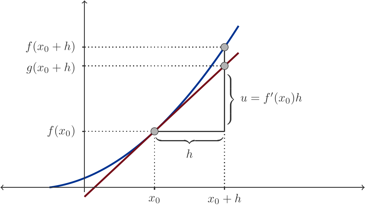
At the beginning, we will explain the equation \(u=f'(x_0)h\) hinted at in Figure 3.9.
Since the tangent \(g\) is a straight line, it has a constant slope. If we read the slope over the interval \([x_0,x_0+h]\), then we obtain the value \(\frac{u}{h}\). On the other hand, the slope of the tangent is equal to \(f'(x_0)\), and thus it follows that \[ \begin{gathered} \frac{u}{h}=f'(x_0)\quad\text{or}\quad u=f'(x_0)h. \end{gathered} \] Our next goal is now to approximate the function value of \(f(x_0+h)\) starting from \(f(x_0)\). For this purpose, we move along the tangent \(g\) to the point \((x_0+h,g(x_0+h))\). The function value of the tangent at \(g(x_0+h)\) is simply \[ \begin{gathered} g(x_0+h)=f(x_0)+u=f(x_0)+f'(x_0)h. \end{gathered} \] Since we have assumed that the distance \(h\) is small, we are near \(x_0\) at the location \(x_0+h\), and therefore we can neglect the difference between \(g(x_0+h)\) and $f(x_0+h): It is significantly smaller than the distance \(h\). We can therefore say \[ \begin{gathered} f(x_0+h) \approx f(x_0)+f'(x_0)h. \end{gathered} \tag{3.28}\] This is the simplest mathematical formulation of the principle of local linearization.
A tangent to the function graph is itself a function graph, specifically, the graph of a particular linear function. This function is \[ \begin{gathered} g(x)=f'(x_0)(x-x_0)+f(x_0). \end{gathered} \tag{3.29}\] Among all possible linear functions \(h(x)=ax+b\), the function \(g\) is distinguished by two properties:
It holds true that \(g(x_0)=f(x_0)\), meaning \(g\) has the same function value at the point \(x_0\) as \(f\).
It holds true that \(g'(x_0)=f'(x_0)\), meaning \(g\) has the same derivative at the point \(x_0\) as \(f\).
The principle of local linearization can now be summarized as follows:
Theorem 3.38 (Local Linearization) If a function \(f(x)\) is differentiable at a point \(x_0\), then it can be approximated locally (near \(x_0\)) by the linear function (3.29).
It is very important for the following to understand the principle of local linearization well. Therefore, we will look at it from several different perspectives in the following.
3.3.4 Marginal Change
In the terminology of economics, derivatives of economic functions are often referred to as marginal concepts. The derivative of a cost function is called marginal cost, the derivative of a revenue function is called marginal revenue, and so on. In interpreting these marginal concepts, reference is often made to the corresponding marginal terms.
This connection between marginal concepts will now be explained in more detail.
Marginal costs are the additional costs incurred by the production of an additional unit of output; marginal revenue is the additional revenue generated by a price increase of one unit of currency. Generally, by marginal change of a function \(f\) at the point \(x\), one understands the change \(f(x+1)-f(x)\) that occurs when the variable is increased by one unit.
The identification of a marginal concept with the corresponding marginal term is based on the possibility of local linearization.
If in equation (3.28) the difference between \(x\) and \(x_0\) is exactly 1 the result for a function differentiable at \(x_0\) is \[ \begin{gathered} f(x)-f(x_0)\approx f'(x_0). \end{gathered} \tag{3.30}\] However, this approximation is only useful if, on the scale with which the variable \(x\) is measured, the difference 1 represents a small change.
Cost Functions
Let \(C(x)\) be the cost function of a manufacturing company. We assume that the cost function is nonlinear. Later in this chapter, we will get to know such examples of nonlinear cost functions.
The marginal unit cost is understood as the cost caused by the production of an additional unit. If \(x_0\) is the currently produced quantity, then the marginal unit cost is \[ \begin{gathered} C(x_0+1)-C(x_0). \end{gathered} \] This is the difference of the function values of the cost function between \(x=x_0+1\) and \(x_0\). Typically, the produced quantity \(x_0>0\) is a large number, compared to which a single unit is a very small change. If the cost function is differentiable, we can therefore approximate the marginal unit cost with local linearization: \[ \begin{gathered} C(x_0+1)-C(x_0)\approx C'(x_0)(x_0+1-x_0)=C'(x_0). \end{gathered} \tag{3.31}\] Since the difference between \(x=x_0+1\) and \(x_0\) is exactly 1, we get the derivative as an approximate value for the marginal unit costs. In economic terminology, the derivative of the cost function is known as marginal cost. Equation (3.31) allows us to approximately equate marginal costs and marginal unit costs.
Exercise 3.39 A cost function is given by \(C(x)=0.03x^2-0.9x+650\). What are the marginal costs and the average costs (cost per unit of output) at a production level of \(x=1000\)?
Solution: The derivative of the cost function is \[ \begin{gathered} C'(x)=0.06x-0.9. \end{gathered} \] Therefore, the marginal costs for \(x=1000\) are \(C'(1000)=59.1\) currency units per unit of output. The average costs are \[ \begin{gathered} \overline{C}(x)=\frac{C(x)}{x}=0.03x-0.9+\frac{650}{x}. \end{gathered} \] Thus, the average costs for \(x=1000\) are \(\overline{C}(1000)=29.75\) currency units per unit of output. □
3.3.5 Relative Change Rate
We now apply the concept of relative difference to the analysis of functions. To measure the change in function values over an interval, we have so far always used the difference in the values at the endpoints of the interval. Instead of the difference in function values, one can also use the relative change in function values as a measure. This is particularly important if the values of the function \(f(x)\) are interpreted as a size whose differences should sensibly be measured by relative differences.
Definition 3.40 Let \(f(x)>0\) be a real function and \([x_1,x_2]\) an interval that is completely contained within the domain of \(f\). The relative or percentage change of \(f\) on the interval \([x_1,x_2]\) is defined as \[ \begin{gathered} r=\frac{f(x_2)-f(x_1)}{f(x_1)}=\frac{f(x_2)}{f(x_1)}-1. \end{gathered} \tag{3.32}\]
The relative change measures the percentage by which \(f(x)\) changes when \(x\) moves from the value \(x_1\) to \(x_2\). Given the relative change \(r\), we have \[ \begin{gathered} f(x_2)=f(x_1)+rf(x_1)=(1+r)f(x_1). \end{gathered} \tag{3.33}\]
Now let \(y=f(x)\) be a differentiable function. As we have seen in Section 3.1.1, the practical significance of the derivative of a function \(f(x)\) lies in the fact that it can convert small changes in \(x\) into the corresponding changes in \(f(x)\). But with what measure can we convert small changes in \(x\) into the corresponding relative (percentage) changes in \(f(x)\)?
We advance the answer and give the explanation for it afterward.
Definition 3.41 If \(f(x)>0\) is a differentiable function on an interval and \(x_0\) is an interior point of the interval, then the quantity \[ \begin{gathered} c:=\frac{f'(x_0)}{f(x_0)}=\left(\ln f(x)\right)'\Big|_{x=x_0} \end{gathered} \tag{3.34}\] is called the (instantaneous) relative change rate of the function \(f(x)\) at the point \(x_0\).
In other words: \(c\) is the logarithmic derivative of \(f(x)\) at the point \(x_0\), which we have already encountered in the formula (3.24).
Now we want to explain why the relative change rate solves the problem formulated at the beginning. Through local linearization, we obtain \[ \begin{gathered} f(x)\approx f(x_0)+f'(x_0)(x-x_0), \end{gathered} \] and from this follows \[ \begin{gathered} \frac{f(x)-f(x_0)}{f(x_0)}\approx \frac{f'(x_0)}{f(x_0)}(x-x_0). \end{gathered} \] Putting \(x:=x_0+h\), we get \[ \begin{gathered} \frac{f(x_0+h)-f(x_0)}{f(x_0)}\approx \frac{f'(x_0)}{f(x_0)}h. \end{gathered} \tag{3.35}\] That means, the relative change rate is exactly that factor \(c\), with which we have to multiply small changes \(h=x-x_0\) in the \(x\)-values, to get the relative change in the function values, thus \[ \begin{gathered} \mbox{$\displaystyle \frac{f(x_0+h)-f(x_0)}{f(x_0)}\approx c\cdot h \quad\mbox{and}\quad f(x_0+h)\approx (1+ch)f(x_0)$}. \end{gathered} \tag{3.36}\]
Let’s summarize again:
The relative change rate \(c=\dfrac{f'(x)}{f(x)}\) indicates the factor by which one can convert (small) absolute changes of \(x\) into the corresponding relative (percentage) changes of \(f\).
Remark 3.42 (Derivative and relative change rate) We now have two quantities available that tell us how strongly a function \(y=f(x)\) changes when the variable \(x\) is altered slightly. The first quantity is the derivative or the instantaneous change rate. It tells us how strongly the function value changes if we measure the function value in the original unit of measure. The second quantity is the (instantaneous) relative change rate. It tells us how strongly the function value changes relatively (in percentage) to the baseline value. The relative change rate is the correct measurement for the instantaneous change of a function \(y=f(x)\) when we describe differences in the variables \(x\) by differences, but differences in the function values by relative differences.
Exercise 3.43 What is the relative growth rate of \(f(x)=2e^{-3x^2}\). What value does it have at the point \(x_0=1\)?
Solution: The relative growth rate is the logarithmic derivative of \(f(x)\). So first we form \(\ln f(x)\). With the rules for logarithms that we have formulated in 2.34 and 2.35, we obtain: \[ \begin{gathered} \ln f(x)=\ln(2e^{-3x^2})= \ln 2-3x^2. \end{gathered} \] With this, we find: \[ \begin{gathered} \left(\ln f(x)\right)'=\left(\ln 2-3x^2\right)'=-6x. \end{gathered} \] At the point \(x_0=1\), \(c\) is \(-6\). □
Exercise 3.44 The GDP of a country grows according to the formula \(f(t)=1200t^{1.2}\). How high is the percentual growth speed at the time \(t=20\)?
Solution: The relative growth rate is obtained as the logarithmic derivative at the point \(t=20\). First, we form: \[ \begin{gathered} \ln f(t)=\ln\left(1200t^{1.2}\right)=\ln 1200 + 1.2\ln t. \end{gathered} \] This gives: \[ \begin{gathered} \frac{f'(x)}{f(x)}=\left(\ln 1200 +1.2\ln t\right)'=\frac{1.2}{t}\,. \end{gathered} \] At the time \(t=20\), it therefore amounts to \(0.06\), which is a growth rate of 6 percent per time unit. □
3.3.6 Exponential growth
In linear functions, the derivative is constant and that is, in a sense, the defining property of linear functions. There are no other functions where the derivative is constant. However, the relative change rate of linear functions is not constant.
But there are also functions where the relative change rate is constant.
Theorem 3.45 Let \(f(x)=Aa^x\) be an exponential function. The relative change rate of this function is \[ \begin{gathered} \frac{f'(x)}{f(x)}=\ln a \quad\mbox{for all $x\in\mathbb R$}. \end{gathered} \]
Proof: This can be easily checked. We know \[ \begin{gathered} \frac{f'(x)}{f(x)}=\left(\ln(Aa^x)\right)'=\left(\ln A+x\ln a\right)'=\ln a. \end{gathered} \] □
The remarkable thing about exponential functions is that their relative change rate is constant. Therefore, exponential functions are as important a class of functions as linear functions. In linear functions, the derivative is constant, in exponential functions, it is the relative change rate that is unchanging.
As we know from (2.37), every exponential function with any base \(a>0\) can be expressed by the exponential function \(\exp(x)=e^x\). It is \[ \begin{gathered} f(x)=Aa^x=Ae^{x\ln a}=Ae^{cx}\quad \mbox{with $c:=\ln a$}. \end{gathered} \tag{3.37}\] Here, the natural logarithm \(\ln a\) appears again, which we originally noted in Theorem 2.58 at this place but at that time could not yet interpret (unless as the nominal interest rate in continuous compounding, see Section 2.6.2). Now we know that it is simply the relative change rate. We can therefore describe a function of the form \[ \begin{gathered} f(x)=Ae^{cx} \end{gathered} \tag{3.38}\] quite simply in words: The initial value is \(f(0)=A\) and the relative change rate is constant and amounts to \(c\). This tells us everything about the function \(f\).
Assume that the relative growth rate of a population is constant at \(c=0.17\), i.e., the population grows by the same percentage in equal time intervals. Then we can describe the changing population number by an exponential function with the relative change rate \(c=0.17\). It must therefore hold that \[ \begin{gathered} f(t)=Ae^{0.17t}. \end{gathered} \] Thus, we have obtained an exact mathematical model for the temporal development and no longer need to estimate the relative change between two time points through numerical approximations, as we have done before. The relative change between two time points \(t_0\) and \(t\) is now \[ \begin{gathered} r=\frac{f(t)-f(t_0)}{f(t_0)}=\frac{Ae^{0.17t}-Ae^{0.17t_0}}{Ae^{0.17t_0}} =e^{0.17(t-t_0)}-1. \end{gathered} \] Assuming the population is at time \(t_0\) a size of \(f(t_0)=1\) million. If one month goes by, then \(t-t_0=\frac{1}{12}\) and \[ \begin{gathered} r=e^{0.17/12}-1=0.014267\,. \end{gathered} \] Hence, according to (3.33): \[ \begin{gathered} f\Big(t_0+\frac{1}{12}\Big)=(1+r)f(t_0)=1\,014\,267. \end{gathered} \] If half a year goes by, then \[ \begin{gathered} r=e^{0.17/2}-1=0.088717 \end{gathered} \] and therefore \[ \begin{gathered} f\Big(t_0+\frac{1}{2}\Big)=(1+r)f(t_0)=1\,088\,717. \end{gathered} \]
Exercise 3.47 The gross domestic product (GDP) of Austria increased between \(2000\) and \(2010\) from \(214\) billion to \(296\) billion Euros. Assuming the relative growth rate was constant.
What is the relative growth rate?
When will the GDP reach the size of \(370\) billion Euros?
Solution:
(a) Since the relative growth rate is assumed to be constant, we can assume the mathematical model of an exponential function: \[ \begin{gathered} f(t) = A\cdot(1+r)^{t} = A\cdot a^{t} = A\cdot e^{ct}. \end{gathered} \] We identify the initial time point \(2000\) with \(t=0\), thus the initial state is \(A =f(0)= 214\), and the year \(2010\) corresponds to \(t=10\). Our model approach thus leads to a power equation, which we can solve: \[ \begin{aligned} f(t)&=A\cdot a^{t}, \\ f(10)&= 214\cdot a^{10} = 296, \\ a^{10}& = \frac{296}{214}, \\ a& = \left(\frac{296}{214}\right)^{1/10} = 1.032970, \\ c &= \ln\,1.032970 = 0.032438\,.\end{aligned} \] The annual increase is \(r=a-1\simeq 0.033\), so about 3.3%, and the relative growth rate is \(c\simeq 0.032\), which is 3.2%.
(b) We calculate with \(a=1.033\). The question leads to an exponential equation: \[ \begin{gathered} f(t) = A\cdot a^{t} = 214\cdot1.033^{t} = 370, \\[5pt] 1.033^{t} = \frac{370}{214} \quad\implies\quad t = 16.864\simeq 17. \end{gathered} \] The year in which the amount of \(370\) billion is reached, is thus \(2000 + 17 = 2017\). In reality, the GDP of Austria in the year 2017 was 370.16 billion Euros. □
Exercise 3.48 The population of a developing country grows annually by \(3\)%. How strongly must the GDP grow annually so that the income per capita doubles within \(20\) years?
Solution: The population grows according to the model of an exponential function \(B(t) = B(0)\cdot1.03^{t}\). For the GDP, we assume the same model with an unknown growth rate: \(E(t)= E(0)\cdot a^{t}\).
The income per capita is obtained as the quotient: \[ \begin{gathered} \dfrac{E(t)}{B(t)} = \dfrac{E(0)}{B(0)}\cdot\bigg(\dfrac{a}{1.03}\bigg)^{t}. \end{gathered} \] This income per capita is supposed to double within 20 years: \[ \begin{gathered} \dfrac{E(0)}{B(0)}\cdot\bigg(\dfrac{a}{1.03}\bigg)^{20} = 2\cdot \dfrac{E(0)}{B(0)} \quad \Rightarrow \quad \bigg(\dfrac{a}{1.03}\bigg)^{20} = 2. \end{gathered} \] This exponential equation has the solution \[ \begin{gathered} a = 1.03\cdot\sqrt[20]{2} = 1.066323 \; \Rightarrow\; \mbox{Annual growth rate $6.6\%$}, \end{gathered} \] respectively, \[ \begin{gathered} c = \ln\,a = 0.0642 \; \Rightarrow\; \mbox{Relative growth rate $6.4\%$}\,. \end{gathered} \] □
3.3.7 Elasticities
We now know two measures with which we can express the changes of a function, namely the derivative and the relative rate of change. However, there is a third measure that is almost more important for economic applications than the first two.
Let \([x_1,x_2]\) be an interval in the domain of the function \(y=f(x)\). We assume that \(0<x_1<x_2\) and \(f(x)>0\) for the entire interval \([x_1,x_2]\). If we want to compare the relative change of the function values \(f(x)\) with the relative change of the variable \(x\), then we form the ratio number \[ \begin{gathered} \frac{f(x_2)-f(x_1)}{f(x_1)}:\frac{x_2-x_1}{x_1}= \frac{f(x_2)-f(x_1)}{x_2-x_1}\frac{x_1}{f(x_1)}. \end{gathered} \tag{3.39}\] If the function is differentiable and if the interval is very small, then we can replace the difference quotient (i.e., the slope of the secant) with the derivative (the slope of the tangent), and thus we obtain the measure \[ \begin{gathered} \epsilon(x_1):=f'(x_1)\frac{x_1}{f(x_1)}=\frac{f'(x_1)}{f(x_1)}x_1. \end{gathered} \tag{3.40}\] The size (3.39) is therefore apprximately equal to the size in (3.40).
The size \(\epsilon(x)\) also plays a role in the natural sciences, and therefore it derives its name.
Definition 3.49 (Elasticity) Let \(y=f(x)>0\) be a differentiable function on \((0,\infty)\) and let \(x_0>0\). Then the quantity \[ \begin{gathered} \epsilon(x_0):=\frac{f'(x_0)}{f(x_0)}x_0=\left(\ln f(x)\right)' x \Big|_{x=x_0} \end{gathered} \tag{3.41}\] is called the elasticity of \(f\) at the point \(x_0\).
Interpretation
First, we note that the elasticity of a function can again be calculated using the logarithmic derivative, as illustrated by (3.41).
Elasticities play a very important role in economic sciences as responsiveness measures. Therefore, we will look at a second way to explain elasticity.
How can a small relative change of \(x\) be converted into the corresponding relative change of \(f(x)\)? We apply the method of local linearization. Let \(x_0\) be increased by a small percentage \(h\): \[ \begin{gathered} \frac{x-x_0}{x_0}=h \implies x=x_0+hx_0. \end{gathered} \] The size \(h\) is therefore the relative change of \(x\). Then, by local approximation with a linear function \[ \begin{gathered} f(x_0+hx_0)\approx f(x_0)+f'(x_0)hx_0, \end{gathered} \] and therefore \[ \begin{gathered} \frac{f(x_0+hx_0)-f(x_0)}{f(x_0)} \approx \frac{f'(x_0)}{f(x_0)}x_0\cdot h= \epsilon(x_0)\cdot h. \end{gathered} \tag{3.42}\] For example, if \(h=0.01\), that is if \(x_0\) is increased by 1 percent, then \[ \begin{gathered} \frac{f(x_0+0.01\,x_0)-f(x_0)}{f(x_0)} \approx \epsilon(x_0)\cdot 0.01. \end{gathered} \tag{3.43}\] This means: if \(x_0\) is increased by 1 percent, the relative change will be \(\epsilon(x_0)\) percent.
This is summarized in the following overview:
Interpretation of Elasticity
The elasticity of a function indicates the factor by which a relative change of \(x\) can be translated into the corresponding relative change of \(f(x)\).
Let \(q(p)\) be the demanded quantity \(q\) of a product depending on the price \(p\). In general, \(q(p)\) is a decreasing function of the price; that is, \(q'(p)<0\) for \(p>0\).
The price elasticity of demand \[ \begin{gathered} \epsilon(p)=\frac{q'(p)}{q(p)}p \end{gathered} \] is a measure for the reaction of demand to small percentage changes in the price: by how much percent does the demand decrease when there is a (small) percentage change in the price?
Since \(q'(p)<0\), \(\epsilon(p)<0\) for \(p> 0\) as well. If \(-1< \epsilon(p)\le 0\), we say that the demand reacts inelastically to price changes because price changes lead to sub-proportional reductions in demand. However, if \(-\infty<\epsilon(p)\le -1\), then the demand is considered elastic. Consumers react markedly to price increases.
Exercise 3.51 The demand is linear in price with \(q(p)=-0.25p+50\). What is the value of the price elasticity of demand at prices \(p=50, 100, 180\)?
Solution: Using (3.41): \[ \begin{gathered} \epsilon(p)=\frac{-0.25p}{-0.25p+50}=-\frac{p}{200-p}. \end{gathered} \] This yields \[ \begin{gathered} \epsilon(50)=-\frac{1}{3}\approx -0.33,\quad \epsilon(100)=-1,\quad \epsilon(180)=-9. \end{gathered} \] If the price were 180 CU and it were increased by 1 % to 181.8 CU, the demand would decrease by 9 %. □
Exercise 3.52 Calculate the elasticity of \(f\) with respect to \(x\) at the point \(x_0\), where \(f(x) = e^{-10\sqrt{x}}\) and \(x_0=1\).
Solution: We calculate the elasticity from the logarithmic derivative of \(f(x)\): \[ \begin{aligned} \ln f(x) &= \ln\left(e^{-10\sqrt{x}}\right)= - 10\sqrt{x}\\[5pt] \left(\ln f(x)\right)'&= \left(-10\sqrt{x}\right)'=-\frac{10}{2\sqrt{x}}=-\frac{5}{\sqrt{x}} \end{aligned} \] From (3.41) we find: \[ \begin{gathered} \epsilon(x)=\left(\ln f(x)\right)'x=-5\sqrt{x}\quad\text{and}\quad \epsilon(1)=-5. \end{gathered} \] Interpretation, if \(f(x)\) is a demand function: If the price starting from \(x=1\) CU increases by \(1\%\), then the demand decreases by \(5\%\). □
Exercise 3.53 The operating costs \(B\) of an apartment depend on the expenditure for rent \(M\) in the following way: \[ \begin{gathered} B=5\sqrt{1+1.5M}. \end{gathered} \] Calculate the elasticity of operating costs \(B\) with respect to rental expenses \(M\), when they amount to 500 CU.
Solution: The calculation progresses thus: \[ \begin{aligned} \ln B&=\ln\left(5\sqrt{1+1.5M}\right)=\ln 5+\frac{1}{2}\ln(1+1.5M),\\ (\ln B)'&= \frac{1.5}{2(1+1.5M)},\\ \epsilon(M)&=(\ln B)'M=\frac{0.75M}{1+1.5M}\,.\end{aligned} \] At the point \(M=500\), we find the value: \[ \begin{gathered} \epsilon(500)=\frac{0.75\cdot 500}{1+1.5\cdot 500} =0.49933 \end{gathered} \] That \(\epsilon(500)\) is so close to \(1/2\) is by no means a coincidence. □
Constant Elasticity
It is clear to us now that elasticity is an interesting quantity. It is natural to ask: are there functions whose elasticity is constant? For related quantities, namely the derivative and the relative change rate, we already know the answer.
Theorem 3.54 (Constant Elasticity) Let \(f\) be a power function, i.e. \(f(x)=Ax^c\) for \(x>0\). Then the elasticity of this function is \(\epsilon(x)=c\) for all \(x>0\).
Justification: We verify: \[ \begin{gathered} \ln f(x)=\ln\left(Ax^c\right)=\ln A+c\ln x\implies (\ln f(x))'=\frac{c}{x} \end{gathered} \] Therefore, \(\epsilon(x)=\dfrac{c}{x}\cdot x=c\). □
Exercise 3.55 The optimal order quantity \(x\) of a company depends on the storage cost rate \(h\) (CU per item and time unit) in the following way: \[ \begin{gathered} x(h)=\sqrt{\frac{a}{h}}. \end{gathered} \] Calculate the elasticity of the order quantity with respect to the storage cost rate.
Solution: The order quantity \(x(h)\) can be written as: \[ \begin{gathered} x(h)=\left(\frac{a}{h}\right)^{1/2}=a^{1/2}\cdot h^{-1/2}\implies \epsilon(h)=-\frac{1}{2}. \end{gathered} \]
3.4 Curve Discussion
3.4.1 Analysis of Monotonicity Properties
The foundation for many important conclusions that one can draw from the properties of the derivative is the so-called Mean Value Theorem of Calculus.
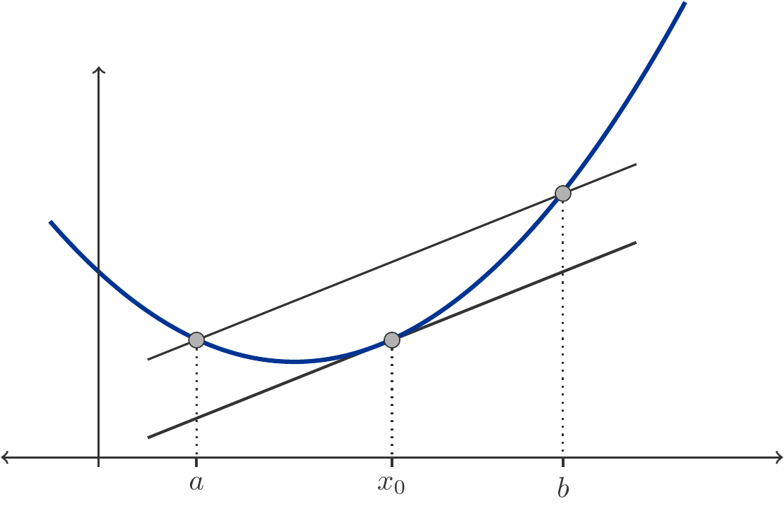
Theorem 3.56 (Mean Value Theorem) If the function \(f\) is continuous on the interval \([a,b]\) and differentiable in the interior, then there exists at least one point \(x_0\) in the interior of the interval such that \[ \begin{gathered} f(b)-f(a)=f'(x_0)(b-a), \end{gathered} \tag{3.44}\] i.e., the derivative is the same as the slope ratio of the function on the interval \([a,b]\).
We forego a strictly formal proof of the Mean Value Theorem. The Mean Value Theorem has a very simple and intuitive interpretation: There exists a point \(x_0\) within the interior of the interval where the tangent is parallel to the connecting line between \((a,f(a))\) and \((b,f(b))\). See also Figure 3.10.
Let us now recall the definition of monotone functions in Section 3.1.1. Since the geometric meaning of the derivative is the slope of the tangent, and because the slope of the tangent visually relates closely to the monotonicity of the function, it is reasonable to draw conclusions about the monotonic behavior of the function from the sign of the derivative.
We have essentially done this often by interpreting the derivative approximately as marginal change. The following theorem repeats these connections.
Theorem 3.57 Let \(f\) be a differentiable function on an open interval \((a,b)\).
If \(f'(x)>0\) for \(x\in (a,b)\), then \(f(x)\) is strictly increasing on \((a,b)\).
If \(f'(x)<0\) for \(x\in (a,b)\), then \(f(x)\) is strictly decreasing on \((a,b)\).
Justification: Let \(f'(x)>0\) for \(x\in (a,b)\). If \(x,y<b\) are two arbitrary points in \((a,b)\) with \(x<y\), we need to show that \(f(x)<f(y)\).
According to the Mean Value Theorem, there is a point \(x_0\) such that \[ \begin{gathered} f(y)-f(x)=f'(x_0)(y-x). \end{gathered} \] Since \(f'(x_0)>0\) and \(y-x>0\), it follows that \(f(y)-f(x)>0\) and therefore \(f(y)>f(x)\). □
Thus, one can infer from the sign of the first derivative whether the function \(f\) is increasing or decreasing.
For an interval \((a,b)\) that contains a point \(x\) with the property \(f'(x)=0\), a statement about the monotonicity is not immediately possible. At such points, the graph of the function has a horizontal tangent.
Theorem 3.58 (Critical Points) Let \(f\) be a differentiable function on an open interval \((a,b)\) and let \(x\in(a,b)\). If \(f'(x)=0\), then \(x\) is called a critical point of \(f(x)\).
The intuitive significance of critical points is made clear by the following theorem.
Theorem 3.59 Let \(f\) be a differentiable function on an open interval \((a,b)\). Between two adjacent critical points of \(f\) in \((a,b)\), the first derivative does not change its sign.
Justification: The sentence is based on an unproven intermediate value property of derivatives that we use: if \(x_1<x_2\) and \(f'(x_1)\not=f'(x_2)\), then the derivative \(f'(x)\) assumes all values between \(f'(x_1)\) and \(f'(x_2)\) on the interval \((x_1,x_2)\). The mean value theorem also essentially relies on this intermediate value property. Intuitively, the intermediate value property of a derivative is plausible: a derivative cannot change abruptly in a function that is differentiable everywhere, because if it did, this would create a kink, and at that point, the function would not be differentiable.
The justification for the statement of Theorem 3.59 then goes like this: If the sign of the derivative changed between two critical points, there would be points \(x\) and \(y\) with \(f'(x)<0\) and \(f'(y)>0\). Consequently, there must be a point \(x_0\) between \(x\) and \(y\) such that \(f'(x_0)=0\). But that is a critical point and therefore the two critical points \(x\) and \(y\) are not adjacent. □
From Theorem 3.59 we can conclude: If there are two critical points \(x_1<x_2\) between which there is no other critical point, then the function \(f(x)\) on the interval \((x_1,x_2)\) is either strictly monotonically increasing or strictly monotonically decreasing. In other words: The monotonic behavior of a function does not change between two successive critical points.
We call an interval in which the monotonic behavior of a function does not change (where the function is either continuously strictly monotonically increasing or continuously strictly monotonically decreasing) a monotonic interval of the function. Knowledge of monotonic intervals is important for a qualitative description of a function graph.
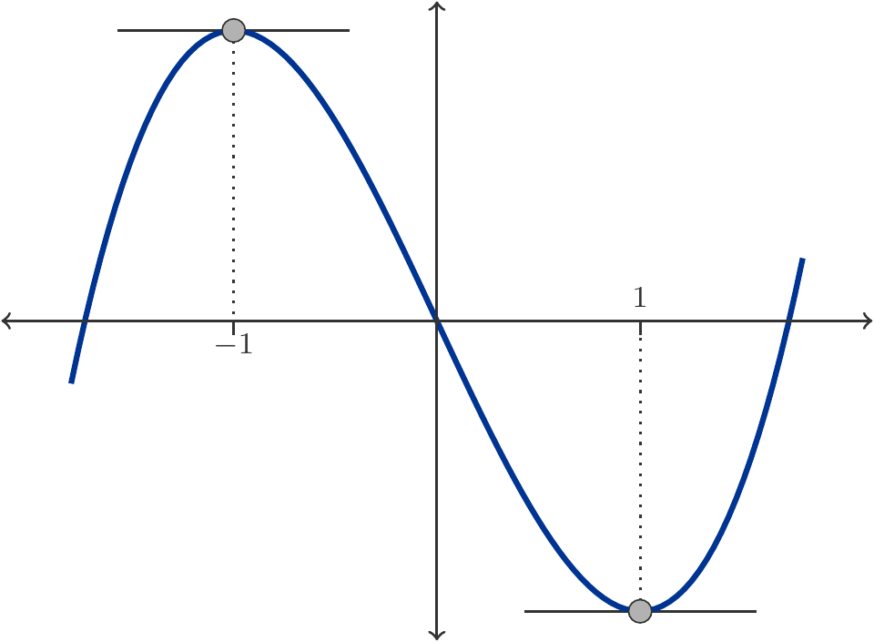
Exercise 3.60 Determine the monotonic intervals of the function \(y=x^3-3x\).
Solution: The derivative of the function is \(f'(x)=3x^2-3\). The critical points with \(f'(x)=0\) are \(x_1=-1\) and \(x_2=1\). These two critical points divide the domain into three intervals: \((-\infty,-1)\), \((-1,1)\), and \((1,\infty)\). In each of these intervals, the function is strictly monotonic.
To determine where the function rises or falls, let’s calculate the derivative at one (arbitrary) point in each of the three intervals, for example at \(x=-2, x=0\) and \(x=2\). We find: \(f'(-2)>0\), \(f'(0)<0\), and \(f'(2)>0\). Thus, the function is strictly monotonically increasing on the interval \((-\infty,-1)\), strictly monotonically decreasing on the interval \((-1,1)\), and again strictly monotonically increasing on the interval \((1,\infty)\), see Figure 3.11. □
At a critical point, the direction of monotonicity can change, but it does not have to. If the direction of monotonicity changes at a critical point, then the critical point is a relative extremum.
Definition 3.61 (Relative Extrema) A critical point \(x_0\) is a relative maximum if at points \(x\) in an open interval around \(x_0\) \[ \begin{gathered} f'(x)=\left\{ \begin{array}{ll} >0 & x<x_0 \\ =0 & x=x_0 \\ <0 & x>x_0 \end{array} \right. \end{gathered} \tag{3.45}\] The critical point \(x_0\) is a relative minimum if at points \(x\) in an open interval around \(x_0\) \[ \begin{gathered} f'(x)=\left\{ \begin{array}{ll} <0 & x<x_0 \\ =0 & x=x_0 \\ >0 & x>x_0 \end{array} \right. \end{gathered} \tag{3.46}\]
Exercise 3.62 Determine the relative extrema of the function \(y=x^4-4x^3+7\).
Solution: The derivative is given by \[ \begin{gathered} f'(x)=4x^3-12x^2=4x^2(x-3). \end{gathered} \] Hence, there are two critical points \(x_1=0\) (a double root of \(f'(x)\)) and \(x_2=3\). Since \(f'(-1)<0\), \(f'(1)<0\) and \(f'(4)>0\), the function is strictly decreasing on both intervals \((-\infty,0)\) and \((0,3)\), and strictly increasing on the interval \((3,\infty)\). Therefore, the critical point \(x_2=3\) is a relative minimum, while the critical point \(x_1=0\) is not a relative extremum, see Figure 3.12.
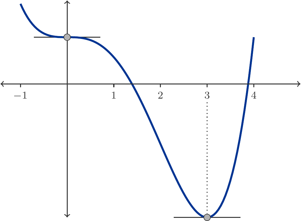
The function has two maximal intervals of monotonicity: On the first monotonic interval \((-\infty,3)\), the function is strictly decreasing. This monotonic interval contains a critical point. On the second monotonic interval \((3,\infty)\), the function is strictly increasing. □
One should not confuse a relative maximum or a relative minimum with an (absolute) maximum (the largest function value) or an (absolute) minimum (the smallest function value). It is possible that a function does not possess a maximum or minimum at all. If an absolute maximum or an absolute minimum exists, then it does not necessarily correspond to a critical point. Consider a strictly monotonic function on a closed interval \([a,b]\): The maximum and minimum are located at the boundaries of the domain interval. Only if the maximum or minimum of a differentiable function is located within the interior of the domain interval, does it also constitute relative extremum points, thus becoming critical points.
We continue with Exercise 3.60 and look for the (absolute) maximum of the function \(f(x)=x^3-3x\) on the interval \([-3,3]\).
The maximum can be a relative maximum or a boundary maximum. The only relative maximum is located at the point \(x=-1\) and equals \(f(-1)=2\). At the boundaries of the domain interval, the function has the values \(f(-3)=-18\) and \(f(3)=18\). Consequently, the function has an absolute maximum at the point \(x=3\). It is a boundary maximum.
3.4.2 Analysis of the Curvature Properties
There are two possibilities for a function graph to be curved. It can be convex or concave. Convex means that the rate of slope is monotonically increasing, while concave means that the rate of slope is monotonically decreasing.
If a function is differentiable, then it is possible to determine the curvature of the function graph by its derivative. This is a convenient method to ascertain whether a function is convex or concave.
Perhaps a small preliminary note is necessary. Until now we have always only considered the derivative of a function \(f\) at a fixed point \(x\), i.e., we have looked at the number \(f'(x)\). But we can also consider \(x\) as a variable and thus arrive at the derivative function \(f':x\mapsto f'(x)\). All concepts that we have available for functions can be applied to the derivative function: One can investigate whether the derivative function is continuous, whether it is differentiable, whether it is monotonic, etc. This concept of derivative as a function will prove to be very useful. The terminology is, however, rather imprecise. People often do not talk about the derivative function when they mean the derivative function \(f'\), but simply call this function the derivative of \(f\). From the context, it is usually clear what is meant.
Theorem 3.64 Let \(y=f(x)\) be a differentiable function on an interval \((a,b)\).
If \(f'\) is strictly monotonically increasing on the interval, then \(f\) is convex on the interval.
If \(f'\) is strictly monotonically decreasing on the interval, then \(f\) is concave on the interval.
Justification: The statement of the sentence is once again intuitively plausible. Since the derivative approximately indicates the slope ratio of the function graph on small intervals, the monotonicity of the derivative is obviously related to the monotonicity of the slope ratio.
An exact proof is based on the mean value theorem. If \(x<y<z\) are three points within the domain of the function \(f\), then according to the mean value theorem there exist intermediate points \(u\in(x,y)\) and \(v\in(y,z)\) such that \[ \begin{gathered} f'(u)=\frac{f(y)-f(x)}{y-x},\quad f'(v)=\frac{f(z)-f(y)}{z-y}. \end{gathered} \] Now, if \(f'\) is strictly monotonically increasing, then \(f'(u)<f'(v)\) and thus \[ \begin{gathered} \frac{f(y)-f(x)}{y-x}<\frac{f(z)-f(y)}{z-y}. \end{gathered} \]
By drawing the graph of the derivative \(f'(x)\), we can determine on which intervals the derivative function \(f'(x)\) is monotonically increasing or decreasing, and from this, we can deduce on which intervals the function \(f(x)\) is convex or concave.
But we can go even further. If the derivative \(f'\) is itself differentiable, then, as we know, the monotonicity properties of \(f'\) are indicated by the derivative \((f')'\). When the derivative \((f')'\) of the derivative function \(f'\) is taken, it results in what is called the second derivative \((f')'=:f''\).
We now summarize the conclusions that we can draw from studying the second derivative:
If the second derivative \(f''\) is positive on an interval, then the first derivative \(f'\) is strictly monotonically increasing there. This implies that the function \(f\) is convex there.
If the second derivative \(f''\) is negative on an interval, then the first derivative \(f'\) is strictly monotonically decreasing and the function \(f\) is concave.
If the second derivative at a point is zero and there is a change in the sign of the second derivative, then the curvature direction of the function \(f\) also changes at that point. This is referred to as an inflection point of the function \(f\).
Curvature can be used to interpret critical points:
Theorem 3.65 (Classification of critical points) Let \(f\) be a function that is differentiable twice and \(x_0\) a critical point. Then: \[ \begin{gathered} f'(x_0) = 0,\quad f''(x_0) < 0 \implies x_0 \text{ is a relative maximum}\\ f'(x_0) = 0,\quad f''(x_0) > 0 \implies x_0 \text{ is a relative minimum} \end{gathered} \]
Justification: If \(f''(x_0)<0\), then there is an interval around \(x_0\) where \(f'\) is strictly monotonically decreasing. Consequently, \(f'(x)>0\) for \(x<x_0\) close to \(x_0\) and \(f'(x)<0\) for \(x>x_0\) close to \(x_0\). Hence, \(x_0\) is a relative maximum.
The second part is proved similarly. □
Exercise 3.66 Determine and classify the critical points of the function \(f(x)=3xe^{-x^2/8}\), see Figure 3.13.
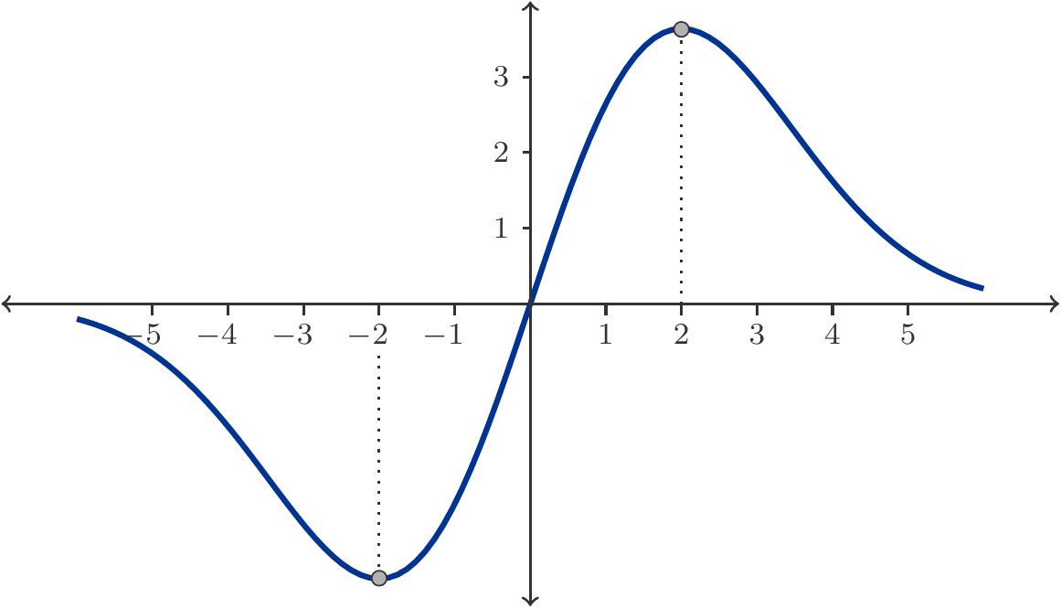
Solution: We form the 1st derivative: \[ \begin{gathered} f'(x)=3e^{-x^2/8}+3x\left(-\frac{2x}{8}\right)e^{-x^2/8}=\frac{3}{4}e^{-x^2/8} (4-x^2). \end{gathered} \] The 1st derivative takes the form of a product, where the first factor, being an exponential function, can never be zero. Thus, by setting the second factor to zero we get: \[ \begin{gathered} 4-x^2=0\implies x_1=-2, \quad x_2=2. \end{gathered} \] Therefore, the function has critical points at \(x=\pm 2\).
We also need the second derivative \(f''(x)\). After some calculation we find: \[ \begin{gathered} f''(x)=-\frac{3x}{16}(12-x^2)e^{-x^2/8}. \end{gathered} \] It follows that: \[ \begin{gathered} f''(-2)=3\cdot e^{-1/2}>0\implies \text{rel. minimum at }x=-2, \end{gathered} \] and \[ \begin{gathered} f''(2)=-3\cdot e^{-1/2}<0\implies \text{rel. maximum at }x=2. \end{gathered} \] □
3.5 Applications – Optimization
Determining relative maxima and minima is a straightforward example of solving nonlinear optimization problems. We now wish to discuss some economic examples of such optimization problems.
3.5.1 Profit optimization under perfect competition
Let \(p\) be the fixed price that a price-taker has to account for in a competitive market. If \(C(x)\) is the cost function of the price-taker, then his profit is \[ \begin{gathered} \pi(x)=px-C(x). \end{gathered} \] With a linear cost function \(C(x)=kx+d\), and if \(p>k\) (the selling price is higher than the per-unit cost), then there is precisely one break-even point \(x=x_0\), from which on the profit is positive. The profit then increases with the quantity produced \(x\) and is only limited by the producer’s capacity. Profit optimization does not make sense in this case.
However, if the cost function is nonlinear, then quite different conditions may exist. For example, the cost function may have the form \[ \begin{gathered} C(x)= V(x)+d, \end{gathered} \] where the variable cost \(V(x)\) is now nonlinear. If such a situation exists, then it may very well be that the obtainable profit must be optimized by choosing a suitable quantity of production.
Exercise 3.67 A manufacturing company is capable of selling any amount of its product at a price of 10,000 monetary units per piece (market price). The cost function is: \[ \begin{gathered} C(x)=\frac{x^3}{10}-60x^2+10000x+1200000. \end{gathered} \] Which production quantity maximizes the profit?
Solution: The profit function (Figure 3.14) is given by \[ \begin{aligned} \pi(x)&=R(x)-C(x)\\ &=10000x-\left(\frac{x^3}{10}-60x^2+10000x+1200000\right)\\ &=-\frac{x^3}{10}+60x^2-1200000.\end{aligned} \]
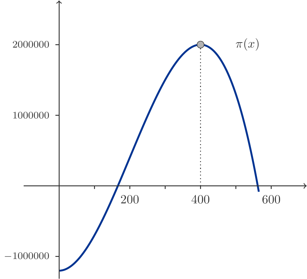
Its first derivative is: \[ \begin{gathered} \pi'(x)=-\frac{3x^2}{10}+120x = -\frac{3x}{10}(x-400). \end{gathered} \] From \(\pi'(x)=0\) we derive the two critical points \(x_1=0\) and \(x_2=400\).
The second derivative \[ \begin{gathered} \pi''(x)=-\frac{3x}{5}+120 \end{gathered} \] has values of \(\pi''(0)=120\) and \(\pi''(400)=-120\) at the critical points. Consequently, \(x_2=400\) is a relative maximum.
Considering the boundary maximum of the domain \([0,\infty)\), only \(x_2=400\) is plausible. Since \(\pi(400)=2000000\) and \(\pi(0)=-1200000\), the relative maximum at \(x_2=400\) is also the absolute maximum. Hence: The profit is maximized by producing 400 units. □
3.5.2 The Break-even point
Another question in the framework of price-taking under perfect competition relates to the minimum price \(p\) at which an offer is still made. When the cost function is linear, the answer to this question is straightforward: The price \(p\) must be higher than the unit costs. However, if the cost function is nonlinear, the matter becomes more complicated and essentially leads back to an optimization problem.
In the short term, a price-taker can forgo covering their fixed costs. Under all circumstances, however, the revenue should cover the variable costs. Therefore, it must hold that: \[ \begin{gathered} \text{Revenue} - \text{variable costs} \ge 0, \\ px-V(x)\ge 0 \implies p\ge \frac{V(x)}{x} =\overline{V}(x)= \text{average variable costs}. \end{gathered} \]
The price must therefore always be at least as high as the average variable costs.
The break-even point is defined as the quantity at which these average variable costs are minimal. The level of these minimum average variable costs is then at the same time the minimum price at which an offer comes about at all: \[ \begin{gathered} p_{\min}=\overline{V}(x_{\min}). \end{gathered} \]
Exercise 3.68 What are the break-even point and the minimum price for a price-taker with the cost function \[ \begin{gathered} C(x)=\frac{x^3}{10}-60x^2+10000x+1200000\;? \end{gathered} \]
Solution: The average variable costs amount to \[ \begin{gathered} \overline{V}(x)=\frac{1}{x}\left(\frac{x^3}{10}-60x^2+10000x\right) =\frac{x^2}{10}-60x+10000. \end{gathered} \] This is a quadratic function whose minimum occurs at the vertex: \[ \begin{gathered} x_{\min}=\frac{60}{2/10}=300, \\[5pt] p_{\min}=\overline{V}(300) =1000\,\text{GE}, \end{gathered} \] where \(p_{\min}=1000\) is the minimum price that must be achieved in order for a company to be willing to act as a supplier at all. □
3.5.3 Pricing Policy of a Monopolist
We have already dealt with the pricing policy of a monopolist several times. Now we are in a position to address related issues in a very general way.
A monopolist is able to vary the price \(p\). He is confronted with a market response, summarized by the demand function \(D(p)\). The monopolist’s revenue amounts to \[ \begin{gathered} R(p)=pD(p), \end{gathered} \] and his profit amounts to \[ \begin{gathered} \pi(p)=R(p)-C(D(p))=pD(p)-C(D(p)), \end{gathered} \] where \(C(x)\) denotes the (possibly nonlinear) cost function.
When optimizing profits, it is sometimes inconvenient to specify the profit function \(\pi\) as a function of the price. The reason for this inconvenience is that it can be laborious to combine a nonlinear cost function \(C(x)\) with the demand function \(D(p)\). It is then usually much easier to represent the profit as a function of the quantity sold.
Exercise 3.69 A company, due to a patent, has a monopoly on an active ingredient demanded by the pharmaceutical industry. The demand function for this product at a price \(p\) is: \[ \begin{gathered} D(p): x=200 e^{-0.01p}\qquad 0<x<200;\text{ $x$ in tons}. \end{gathered} \] The production costs are a linear function of the output quantity \(x\): \[ \begin{gathered} C(x)=1500+50x. \end{gathered} \]
What profit does the company make if it maximizes its revenue?
What is the maximum profit the company can achieve?
Solution: To maximize revenue, we could represent the revenue function as a function of price as before. However, since we also want to calculate the profit achieved, we will immediately switch to representing it as a function of the quantity sold.
We calculate the inverse demand function, which is the function that tells us the price \(p\) for any quantity \(x\) that would lead to the complete sale of that quantity \(x\): \[ \begin{gathered} D(p): x=200 e^{-0.01p}\quad\implies \quad D^{-1}(x): p=-100\ln x+100\ln(200). \end{gathered} \] Therefore, the revenue function takes the following form: \[ \begin{gathered} R(x) = p \cdot x = -100 x \ln x + 100 x \ln(200).\qquad \mbox{(A)} \end{gathered} \] The profit function is: \[ \begin{aligned} \pi(x)&=R(x)-C(x)\\[5pt] &=-100x\ln x+100x\ln(200)-50x-1500.\qquad \mbox{(B)} \end{aligned} \] (a) To find the revenue maximum, we calculate the marginal revenues \(R'(x)\) (using the product rule!): \[ \begin{aligned} R'(x)&= -100\ln x-100+100\ln(200)\\[5pt] &=-100\left(\ln x+1-\ln(200)\right). \end{aligned} \] Setting the marginal revenues to zero, i.e., \(R'(x)=0\), we get the equation: \[ \begin{gathered} \ln x+1-\ln(200)=0\implies \ln x=\ln(200)-1. \end{gathered} \] This equation has a unique solution: \[ \begin{gathered} x=e^{\ln(200)-1}=\frac{200}{e}\simeq 73.58. \end{gathered} \] This is indeed the maximum of the revenue function, because \[ \begin{gathered} R''(x)=-\frac{100}{x}<0\quad\text{for all }x>0. \end{gathered} \] What profit does the company achieve with this strategy?
We substitute \(x=200/e\) into the profit function, keeping in mind: \[ \begin{gathered} \ln\left(\frac{200}{e}\right)=\ln(200)-1. \end{gathered} \] Thus we obtain: \[ \begin{aligned} \pi\left(\frac{200}{e}\right)&=-\frac{20000}{e}\left(\ln(200)-1\right) +\frac{20000}{e}\ln(200)-\frac{10000}{e}-1500\\[5pt] &=\frac{10000}{e}-1500\simeq 2178.8 \text{ CU}. \end{aligned} \]
(b) We now consider the second strategy, which is undoubtedly guided by commercial caution: we form the first derivative of the profit function (given in (B)) and set it to zero: \[ \begin{aligned} \pi'(x)&=-100\ln x-150+100\ln(200) = 0,\\[5pt] \ln x&=\ln(200)-\frac{3}{2}\implies x=\frac{200}{e^{3/2}}\simeq 44.626. \end{aligned} \] The readers can easily verify that \(\pi''(x)=-100/x\). The profit function therefore has a unique maximum at \(x=200/e^{3/2}\). The profit achieved with this sales volume is: \[ \begin{aligned} \pi\left(\frac{200}{e^{3/2}}\right)&=\frac{20000}{e^{3/2}}-1500\simeq 2962.6 \end{aligned} \] □
3.5.4 Optimal Inventory Management
As another application, we look at a famous problem from inventory theory, the Economic Order Quantity model (EOQ).
Imagine a trading company that distributes a product, which it must obtain from a manufacturer itself. This product is stocked in sufficient quantities to meet customer demand.
Furthermore, we assume that demand is constant in the sense that the product is removed from inventory at a constant rate \(\lambda\). The rate \(\lambda\) is measured in units or QU per unit of time.
At certain intervals, new orders are placed with the manufacturer of the product, the ordered quantities are delivered and added to the current inventory level \(I(t)\) at time \(t\).
How does the inventory level \(I(t)\) develop over time? In Figure 3.15, a typical inventory trend is graphically represented.
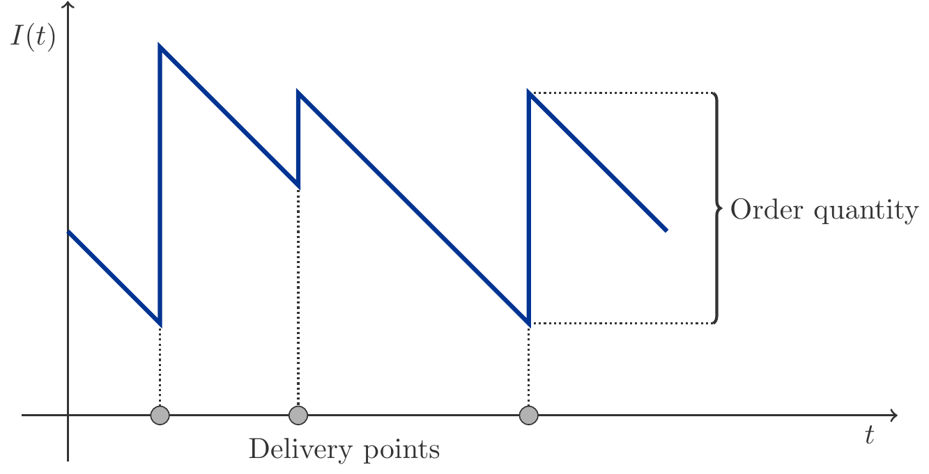
This is a very peculiar, sawtooth-like pattern, which can be explained as follows:
The function \(I(t)\) has jump discontinuities at the delivery points. The height of the jumps corresponds to the delivered quantities. In the simplest version of the EOQ model, it is assumed that what was ordered is also delivered.
Between the jump discontinuities, \(I(t)\) decreases linearly with a slope of \(-\lambda\), as it is assumed that the product is removed from inventory at a constant rate.
If we assume a simple, yet plausible cost structure, which we will discuss shortly, it turns out that the inventory pattern in Figure 3.15 is not optimal.
Intuitively speaking, optimality in terms of lowest possible costs is achieved by calming the somewhat erratic image of the inventory function \(I(t)\) as much as possible. This is achieved by:
Always ordering the same quantity \(x\).
Timing the orders such that a new delivery arrives just when the inventory level would drop to zero.
This results in an ideal inventory pattern, as shown in Figure 3.16.
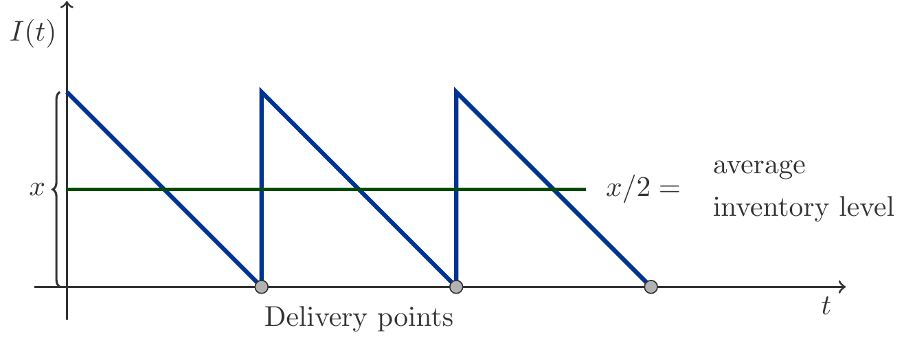
The EOQ model is based on the following simple cost structure:
Each ordering process causes fixed costs \(K\), independent of the order quantity \(x\).
The ordered product must be paid for at the supplier, with a purchase price of \(c\) currency units per item.
The delivered quantities have to be stored, which incurs costs for the actual physical storage (holding cost) of \(h\) (currency units per item and per unit of time).
Now, we commit to a unit of time, for example, one year3.
The total costs \(C(x)\) for an order quantity \(x\) are as follows:
With an annual demand of \(\lambda\) items, \(\lambda/x\) ordering processes are required. This results in a cost contribution of \(K\lambda/x\).
The demand \(\lambda\) has to be paid to the supplier, incurring costs of \(c\lambda\).
Since the inventory level decreases uniformly, meaning linearly from \(x\) to 0, the average inventory level is \(x/2\), half the height of the sawtooth. Therefore, the average cost for physical storage is \(hx/2\).
This leads to the total cost per unit of time for an order quantity \(x\): \[ \begin{gathered} C(x)=\frac{K\lambda}{x}+c\lambda+h\,\frac{x}{2}. \end{gathered} \tag{3.47}\] We are looking for the optimal order quantity \(x^\ast\), which ensures a minimum of (3.47). We proceed as usual: \[ \begin{aligned} C'(x)=-\frac{K\lambda}{x^2}+\frac{h}{2}=0. \end{aligned} \] This simple quadratic equation has a positive solution: \[ \begin{gathered} x^\ast=\sqrt{\frac{2K\lambda}{h}}\,. \end{gathered} \tag{3.48}\] This is the famous Wilson-Harris Formula for the optimal order quantity in the EOQ model. With the help of \(x^\ast\), we can also easily calculate at what intervals orders should ideally be placed. To do this, we simply divide the optimal order quantity by the demand \(\lambda\): \[ \begin{gathered} t^\ast=\frac{x^\ast}{\lambda}=\sqrt{\frac{2K}{h\lambda}}. \end{gathered} \tag{3.49}\] That \(x^\ast\) is indeed a minimum can be seen from the second derivative: \[ \begin{gathered} C''(x)=\frac{2K\lambda}{x^3}>0\quad\text{for all }x>0. \end{gathered} \]
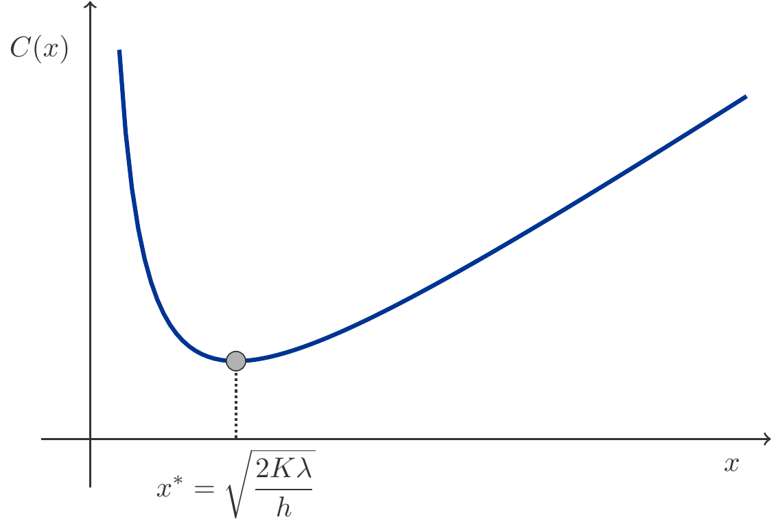
Exercise 3.70 A trading company distributes a product of which 50,000 units are sold per year. The storage costs are 0.4 monetary units (MU) per piece per year. The purchase price is 4 MU per piece, and the fixed costs of a procurement process are 400 MU.
What is the optimal order quantity?
How many times per year must an ordering process be carried out?
What is the optimal interval (in days) between orders?
Solution: Let’s choose 1 year as the time unit. From the given information we have: \[ \begin{aligned} %% {alignat*}{2} \lambda &=50000 &\quad & \text{Demand}\\ K&=400 & & \text{order fixed costs}\\ c&=4 && \text{purchase price}\\ h &= 0.4 && \text{storage cost rate}\end{aligned} \] This results in the cost function (3.47): \[ \begin{gathered} C(x)=\frac{K\lambda}{x}+c\lambda+h\,\frac{x}{2}=\frac{20000000}{x} +200000 + 0.2x,\\ C'(x)=-\frac{20000000}{x^2}+0.2 =0,\\ x_1=-10000,\quad x_2=10000. \end{gathered} \] The optimal order quantity is therefore \(x^\ast=10000\) units.
Since the annual demand is 50,000 units, there must be \(50000/10000=5\) ordering processes per year.
The optimal time interval between two orders is \[ \begin{gathered} t^\ast =\frac{x^\ast}{\lambda}=\frac{10000}{50000}=0.2\ years = 73\ days. \end{gathered} \] □
Exercise 3.71 An electronics shop, among other things, sells flat screens (55-inch diagonal) with a purchase price of 348 MU. On average, 1900 of these devices are sold per week. The storage cost per device is 2.40 MU per piece per week. An order process with the manufacturer of the devices incurs personnel costs of 1200 MU and handling costs (transport, etc.) of 2430 MU. The company expects financing costs of 9% per year (lost interest for the capital value of stored goods).
What amount of flat screens should be ordered with each order process so that the total storage costs are minimized?
At what intervals should these orders be placed?
Solution: We calculate with a time unit of 1 week. Note that the interest rate is an annual interest rate which must be accordingly converted.
(a) The demand per week is \(\lambda=1900\) units. Let’s first list the fixed costs \(K\) and the variable costs \(c\) per order process: \[ \begin{aligned} K&=\text{handling costs}+\text{personnel costs}\\ &=1200+2430 =3630, \\ c&=\text{purchase price}=348. \end{aligned} \] For storage cost rate \(h\): it consists of costs for the physical storage of devices plus the lost interests for the capital tied up in stock: \[ \begin{aligned} h&=2.4+348\cdot \frac{0.09}{52}=3.0023\,. \end{aligned} \]
The total costs with an order quantity \(x\) are then: \[ \begin{aligned} C(x)&=\frac{K\cdot \lambda}{x}+c\cdot \lambda+\frac{h}{2}\cdot x \\ &=\frac{3630\cdot 1900}{x}+348\cdot 1900+3.0023\cdot \frac{x}{2}\,. \end{aligned} \] These total costs are minimal for the order quantity \[ \begin{gathered} x^\ast=\sqrt{\frac{2K\lambda}{h}} =\sqrt{\frac{2\cdot 3630\cdot 1900}{3.0023}} =2143.5\,. \end{gathered} \]
(b) The optimal order interval results from: \[ \begin{gathered} t^\ast=\frac{x^\ast}{\lambda}=\frac{2143.5}{1900} = 1.1281\ weeks \simeq 8\ days. \end{gathered} \] □
3.5.5 Further Optimization Problems
Exercise 3.72 (Useful Life of an Investment) The purchase costs of a machine are 300,000 MU, and the operating costs increase annually by 25,000 MU starting from 25,000 MU in the first year. What useful life causes the lowest average total costs?
Solution: The operating costs of the individual years form an arithmetic sequence with a sum \(B(n)\) over the first \(n\) terms. These are the accumulated total operating costs after the \(n\)-th year of operation. We have \[ \begin{gathered} B(1)=25000,\quad B(n)=25000+25000(n-1)=25000n. \end{gathered} \] Using the sum formula (1.8): \[ \begin{gathered} S(n)=\frac{n}{2}(B(1)+B(n))=12500n(n+1). \end{gathered} \] Thus, the total costs after the usage time \(t\) are (we set \(n=t\)): \[ \begin{gathered} C(t)=300,000+12,500t+12,500t^2. \end{gathered} \] It is necessary to determine that usage time \(t\) for which the average costs \[ \begin{gathered} \overline{C}(t)=\frac{C(t)}{t}=\frac{300,000}{t}+12,500+12,500t \end{gathered} \] are minimal.
We calculate the first derivative and set it to zero: \[ \begin{gathered} \overline{C}'(t)=-\frac{300000}{t^2}+12500=0,\\ t =\sqrt{\frac{300000}{12500}}= 4.899\ years. \end{gathered} \] □
Someone acquires an asset at a purchase cost of \(I_0\) MU (monetary units) with the intention to sell it later. The resale value \(R(t)\) is a known function of time \(t\).
What is the optimal time \(T\) to sell the asset, assuming that owning the asset does not incur significant costs?
Under what conditions does such an optimal selling time exist?
To determine \(T\), we argue as follows: the profit from selling at time \(t\) is the difference between \(R(t)\) and the accumulated value \(I_0e^{ct}\), if the initial investment \(I_0\) had been put into an alternative investment with an interest rate \(c\) (continuous compounding). Equivalently, the present value of the profit can be obtained by discounting: \[ \begin{gathered} \pi(t)=R(t)e^{-ct}-I_0. \end{gathered} \] We take the first derivative and set it to zero: \[ \begin{gathered} \pi'(t)=e^{-ct}\left(R'(t)-cR(t)\right)=0. \end{gathered} \] Since \(e^{-ct}>0\), a critical point \(t\) must satisfy the equation \(R'(t)-cR(t)=0\). It follows: \[ \begin{gathered} \frac{R'(t)}{R(t)}=c. \end{gathered} \tag{3.50}\] This condition is interesting, as it states that the relative rate of change of the resale value must equal the interest rate of the alternative investment.
Let \(T\) be a solution to (3.50), hence \(R'(T)-cR(T)=0\). In order for there to be a local maximum at point \(T\), it must be that \(\pi''(T)<0\). \[ \begin{aligned} \pi''(T)&=e^{-cT}\bigg[R''(T)-cR'(T)-c \big(\underbrace{R'(T)-cR(T)}_{=0}\big)\bigg]\\[5pt] &=e^{-cT}\big(R''(T)-cR'(T)\big)<0. \end{aligned} \] This last condition can only be satisfied if \[ \begin{gathered} (R''(T)-cR'(T)<0\implies \frac{R''(T)}{R'(T)}<c \end{gathered} \tag{3.51}\] In other words, a critical point is a maximum exactly when the relative rate of change of \(R'(T)\) is less than the interest rate.
Exercise 3.74 An investor decides to invest 10,000 MU in a startup company. Comprehensive statistical analyses regarding the potential of the investment revealed that the most likely scenario is that the value of the investment will increase linearly by 25% per year over the next few years.
What would be an ideal time to sell the investment if there is the possibility to alternatively invest the capital with a guaranteed 10% return risk-free?
Solution: The resale value of the investment is \[ \begin{gathered} R(t)=10000(1+0.25t). \end{gathered} \] The present value of the profit from the sale of the investment at time \(t\) is: \[ \begin{gathered} \pi(t)=10000(1+0.25t)e^{-0.1t}-10000. \end{gathered} \] The condition (3.50) is: \[ \begin{gathered} \frac{2500}{10000(1+0.25t)}=0.1\implies t=\frac{1500}{250}=6. \end{gathered} \] Thus, the optimal time to sell the investment is after \(T=6\) years. That maximum profit is really achieved at this point in time is resulting from the condition (3.51), which is automatically satisfied here. Because \(R''(t)=0<0.1\) for all \(t\), and hence \(R''(t)/R'(t)=0\). A graphical illustration of the more general case of a linear resale value \(R(t)=I_0(a+bt)\) is shown in Figure 3.18. □
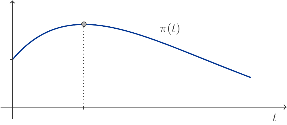
3.6 Additional Exercises
-
Determine the 1st derivative of \(y=3 x^{6}-19 x -9\) at the point \(x=1\).
Solution: \(y'=18x^5-19\), \(y'(1)=-1\).
-
Determine the 1st derivative of \(y=(2x+3)^4\) at the point \(x=0\).
Solution: \(y'=8(2x+3)^3\), \(y'(0)=216\).
-
Determine the 1st derivative of \(y=3x^2e^{-x}\) at the point \(x=1\).
Solution: \(y'=3x(2-x)e^{-x}\), \(y'(1)=1.1036\).
-
Determine the 1st derivative of \(y=(2x-1)^2e^{-x^2/5}\) at the point \(x=0\).
Solution: \(\displaystyle y'=-\frac{2}{5}(10-19x-4x^2+4x^3)e^{-x^2/5}\), \(y'(0)=-4\).
-
Determine the 1st derivative of \(y=\sqrt{10+3^x}\) at the point \(x=0\).
Solution: \(\displaystyle y'=\frac{3^x\ln 3}{2\sqrt{10+3^x}}\), \(y'(0)=0.1656\).
-
Determine the 1st derivative of \(y=\ln(1+\sqrt{x})\) at the point \(x=1\).
Solution: \(\displaystyle y'=\frac{1}{2\sqrt{x}(1+\sqrt{x})}\), \(y'(1)=1/4\).
-
Determine the 1st derivative of \(y=\sqrt{e^{-5x^4}}\) at the point \(x=1\).
Solution: \(\displaystyle y'=-10x^3e^{-5x^4/2},\quad y'(1)=-0.8208\).
-
Determine the 1st derivative of \(y=\ln(x^{3-\sqrt{x}})\) at the point \(x=1\).
Solution: \(\displaystyle y'=-\frac{\ln x}{2\sqrt{x}}+\frac{3-\sqrt{x}}{x}, \quad y'(1)=2\).
-
Determine the 1st derivative of \(y=x^{2x}\) at the point \(x=2\).
Solution: \(y'=2 x^{2x}(\ln x+1),\quad y'(2)=32(1+\ln 2)=54.1807\).
-
Determine the 1st derivative of \(\displaystyle y=\frac{e^{3x}}{1+x}\) at the point \(x=0\).
Solution: \(\displaystyle y'=\frac{e^{3x}(2+3x)}{(1+x)^2},\quad y'(0)=2\).
-
The gross domestic product of a country increased from 696 billion GE to 991 billion GE between 1990 and 2000. It is assumed that the relative growth rate of GDP is constant. What is the relative growth rate?
Solution: 3.53 %
-
Calculate the relative rate of change \(c(x)\) for the function \(f(x)=\sqrt{x}\) at the point \(x=1/2\).
Solution: \(\displaystyle c(x)=\frac{1}{2x},\quad c(1/2)=1\).
-
Calculate the relative rate of change \(c(x)\) for the function \(f(x)=2^{x^2-1}\) at the point \(x=1\).
Solution: \(\displaystyle c(x)=2x\ln 2,\quad c(1)=2\ln 2\simeq 1.3862\).
-
Compute the elasticity of \(f(x)=e^{-8\sqrt{x}}\) at the point \(x_0=7\).
Solution: \(\epsilon(x)=-4\sqrt{x},\;\epsilon(7)=-4\sqrt{7}\simeq -10.58\).
-
Compute the elasticity of \(f(x)=e^{-x^2+5x+3}\) at the point \(x_0=3\).
Solution: \(\epsilon(x)=-x(2x-5),\quad \epsilon(3)=-3\).
-
Compute the elasticity of \(f(x)=(2x-5)^3\) at the point \(x_0=1\).
Solution: \(\displaystyle \epsilon(x)=\frac{6x}{2x-5},\quad \epsilon(2)=-2\).
-
Given is the demand function \(q=250p^{-0.2}\). Calculate the price elasticity of demand.
Solution: \(\epsilon(p)=-0.2\).
-
Given is the demand function \(q=-3p+2400\). In which interval for \(p\) is the demand elastic?
Solution: \(400\le p<800\)
-
Given is the demand function \(q=-\sqrt{p}+3\). In which interval for \(p\) is the demand elastic?
Solution: \(4\le p<9\).
-
Identify and classify the local extrema of the function \(y=x^2e^{-x/2}\).
Solution: Maximum at \(x=4\), minimum at \(x=0\).
-
Identify and classify the local extrema of the function \(y=x\ln x\).
Solution: Minimum at \(x=1/e\simeq 0.3679\).
-
Identify and classify the local extrema of the function \(\displaystyle y=\frac{x-1}{x^2+3x+5}\).
Solution: Minimum at \(x=-2\), maximum at \(x=4\).
-
Identify and classify the local extrema of the function \(y=(2x-1)e^{-x^2}\).
Solution: Minimum at \(x=-1/2\), maximum at \(x=1\).
-
A company produces with the cost function \[ \begin{gathered} C(x)=9x-4x\ln(x+1)+3x^2. \end{gathered} \] Calculate the marginal costs for an output of \(x=10\) units.
Solution: \(\displaystyle C'(x)=9-4\ln(x+1)-\frac{4x}{x+1}+6x,\quad C'(10)\simeq 55.77\).
-
Given is the demand function \(q=25e^{-0.1p}\) of a monopolist. At what price is maximum revenue achieved?
Solution: \(p=10\).
-
A company produces a product that it can sell at a price of 221 CU. The competitive situation does not allow to influence the price over the quantity in the long run. The total production cost for a quantity \(q\) is given by the cost function: \[C(q)= 0.0014 q^3- 0.31q^2+ 24.2515 q+27800.\] What quantity of the product must be sold to achieve maximum profit? Round the result to a whole number.
Solution: \(q\simeq 302\).
-
What is the operating minimum for a price-taking firm with cost function \[ \begin{gathered} C(x)=0.021x^3-34.272x^2+13998x+1100\; ? \end{gathered} \] What is the minimum price that must be achievable in the market for the company to even appear as a supplier?
Solution: \(x_0=816,\quad p_{\min}=15.024\)
-
A chemical company has a monopoly on a specific pesticide due to a patent. The inverse demand function for this product in wholesale is: \[ \begin{gathered} D^{-1}(x): p=- 1.26x+ 349.32\,. \end{gathered} \] Fixed costs of 4411 CU are incurred in production, and the variable costs are given by the function: \[ \begin{gathered} C_v(x)= 0.006x^3- 0.07x^2+ 32.05x\,. \end{gathered} \] What profit does the company make when it maximizes its revenue? Round the result to a whole number.
Solution: 721
-
A monopoly supplier has the inverse demand function \(D^{-1}(q)\) and cost function \(C(q)\) given by \[ \begin{aligned} D^{-1}(q): p & = -0.87q + 260.50,\\ C(q) & = 0.020q^3 - 0.12 q^2 + 36.18 q + 2736 \end{aligned} \] What is the maximum profit the company can achieve? Round the result to a whole number.
Solution: 4105
-
In a monopoly market, the quantity demanded \(x\) depends on the price \(p\) as \(x=4500 p^{-1.2}, p>0\). The monopolist produces with a cost function \(C(x)=5x+1000\). At what sales quantity \(x_0\), and what price \(p_0\) does the monopolist achieve maximum profit? How much is this profit?
Solution: \(x_0=75.97,\quad p_0=30\), profit \(\pi=899.36\).
-
A manufacturer must produce \(144,000\) units per year. The material costs are \(5\) CU per unit, and the fixed costs before each production run amount to \(160\) CU. The storage costs are \(0.5\) CU per piece per year.
Calculate the optimal batch size.
Solution: 9600
-
A household appliance manufacturer also produces refrigerators under the brand Permafrost. These devices are equipped with compressors, the purchase price of which is 111 CU (currency units). On average, 1200 such compressors are needed per week. The storage costs for a compressor are 5.55 CU per week. An order from the manufacturer of the compressors causes personnel costs of 1530 CU and processing costs (transportation, etc.) of 1710 CU. The company calculates with financing costs of 12% per year. Calculate the optimal order quantity. Which ordering interval (in days) guarantees minimum storage costs? Round the result to a whole number.
Solution: \(x^\ast = 1157.2678 \approx 1157, t^\ast=7\cdot 1157.2678/1200 \approx 7\) days.
-
A car manufacturer requires 40000 tires of a specific type per year, which are purchased at a unit price of 60 CU. The fixed costs are 200 CU per order. The costs for storage amount to 10 CU per tire per year. The management currently operates a Just-in-Time inventory policy, meaning the required tires are delivered daily. Production occurs 365 days a year.
By how much could the costs of storage be reduced if the company operated optimal inventory storage?
What would actually be the optimal ordering interval (in days)?
Solution: Cost advantage: 60,899.8 CU, Interval: 12 days.
-
Today (\(t=0\)), you acquired 20 bottles of Mouton Rothschild Tchelitchev vintage 1956 at a total price of 8000 CU. As a wine connoisseur, you know that the resale value \(R(t)\) of this wine evolves according to the following law: \[ \begin{gathered} R(t)=8000(1+0.5t)^{1.2}\qquad t\text{ in years} \end{gathered} \] After how many years should you sell this exquisite wine so that your profit is maximized? Calculate using a nominal annual interest rate of 5% with continuous compounding.
Solution: 22 years
The equation of a straight line through a given point \((x_0,y_0)\) with a given slope \(k\) can be determined by \(\frac{y-y_0}{x-x_0}=k \; \Rightarrow \; y=k(x-x_0)+y_0.\)↩︎
A heuristic argument is not logically compelling, but it serves as a guide for our imagination.↩︎
It is immaterial which time unit we choose, only that it must be consistently used in all calculations!↩︎